X-Plane 11.30 offers to equip planes with preconfigured autopilots, in addition to the many configurable options of previous X-Plane versions. Some of the available autopilots come with additional features. Read More
Comments Off on Preconfigured autopilots and other autopilot changes in 11.30
The X-Plane autopilot works with cascaded PID controllers. Tuning the PID controllers for your aircraft is key to having a smooth working autopilot. This article explains the parameters you can set in Plane Maker, and how to tweak them.
Starting with X-Plane 11.30, it is possible to equip high-flying aircraft with an oxygen system rather than or in addition to the pressurized cabin, to allow realistic black-out behavior also with unpressurized aircraft. Read More
X-Plane simulates ice accumulation on your aircraft that will affect your performance greatly. X-Plane also simulates a wide variety of systems that can prevent the accumulation of ice on various surfaces (anti-ice), or get rid off ice that has accumulated (de-ice). Read More
Comments Off on The X-Plane Anti- and De-Ice systems
X-Plane simulates governors for constant speed propellers that can have various failure modes. Depending on the type of engine/propeller combination on the aircraft, the behavior of the governor in case of an engine failure will be different. X-Plane 11.30 allows you to select the type of governor to simulate, to accommodate a wide range of different engine types. Read More
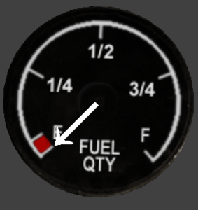
Let’s suppose we are simulating a faulty fuel quantity gauge for a historic plane, the “Arbitria Examplus Mk 2”. The plane had a real fuel capacity of 200kg, but showed empty when there was 5kgs left, and full when there was 190kg in the tank. Plane Maker will provide the sim with the real fuel capacity while this animation will provide the visual realism.
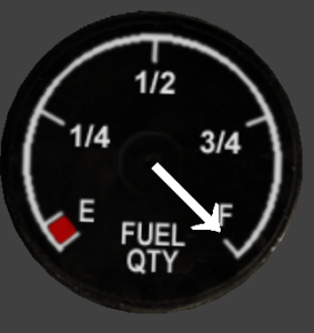
The fuel gauge, at frame 1The fuel gauge, at frame 2
First, we model a gauge and a needle, initially pointed up at 0 degrees. The texture used here is fuel_round_GA.png, included with Plane Maker.
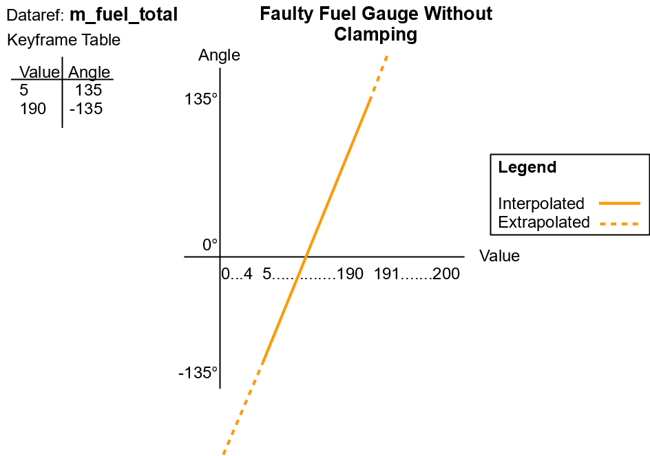
We are using the dataref sim/flightmodel/weight/m_fuel_total. The first keyframe shows the gauge’s arrow at the empty position (135 degrees), and will be shown when the dataref is 5. The second keyframe shows the gauge’s arrow at the full position (-135 degrees), and will be shown when the dataref is 190. Here is a chart of this data as a table and graph of the arrow’s rotation over changes in m_fuel_total.
The faulty fuel gauge animation, in table and graph form, without clamping
When sim/flightmodel/weight/m_fuel_total is between our explicitly created keyframes (5 and 195) it will animate as intended because X-Plane is interpolating between these known keyframes. But, beyond that X-Plane will guess by using the first two keyframes for when the dataref is less than 5 and the last two keyframes when the dataref is greater than 190. (In this case we only have two keyframes, both are used to “look ahead” and “look behind”). This is called extrapolation. Extrapolation is useful as it allows you to animate just a portion of the range of motion and allow X-Plane to do the rest. It is convenient and allows you to think of animation as incremental motion (10 degrees CCW every change of .1) that builds up dynamically rather than one large static motion that will be broken up into chunks.
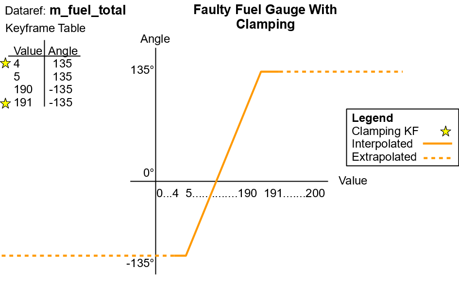
There is currently a problem with our animation! We want the needle to stop moving when it reaches 5kg or 190kg, but this keyframe table will allow X-Plane to keep rotating the needle for all of 0 to 200. X-Plane’s extrapolation cannot be turned off; instead we must trick it using “clamping keyframes”. By using another keyframe on each side of the keyframe table with the same angle and a smaller and larger value respectively, we can “clamp” the animation and stop incorrect extrapolation from ruining our fuel gauge!
The faulty fuel gauge animation, in table and graph form, without clamping
You can see in the graph how the extrapolation is now fooled! By giving X-Plane a flat line to follow, rather than a sloped one, past certain values the angle of rotation will stay the same no matter the dataref’s value. The value for the dataref simply has to be less than or greater than each side, but many artists use a convention to quickly identify what is a clamping keyframe. Some use -999999,999999 or adding or subtracting 1 off each end as we’ve done in this example. Both work equally well, so the real value is in being consistent. Though rarely used, it is also possible to clamp only one side of a keyframe table.
Although a rotating gauge was used, this principle applied to translations as well.
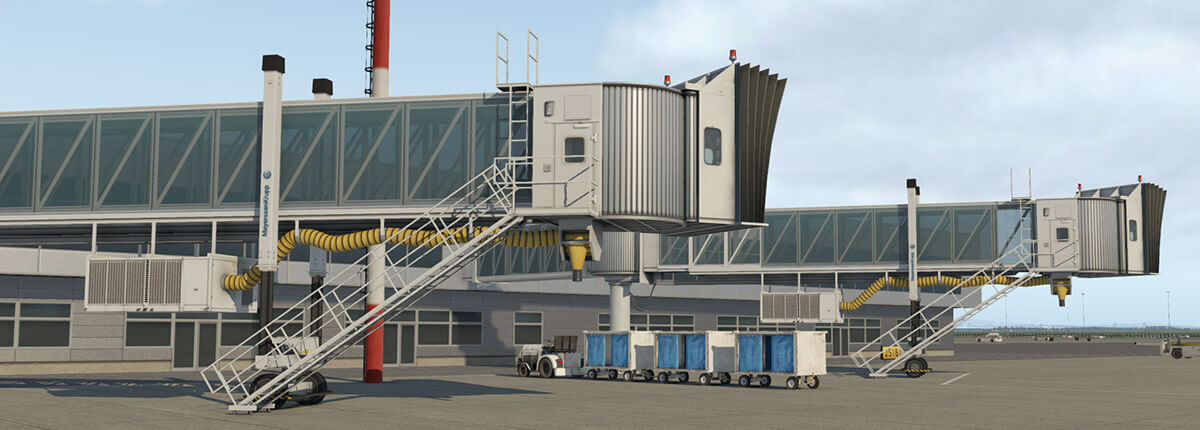
X-Plane 11.20 introduces a new object-type for the construction of jetways. Technically this is a facade, and therefore in WED appears as an unclosed chain of segments. This approach allows the artist to customize jetway shape and position for almost any real world situation. Moreover, it is very easy to use, and you can build a custom jetway literally with just a few steps.
The jetway system can handle an unlimited number of extension bridges in a single chain, and telescopic bridges in a range of 11 to 40 meters. By design, jetways are always horizontal.
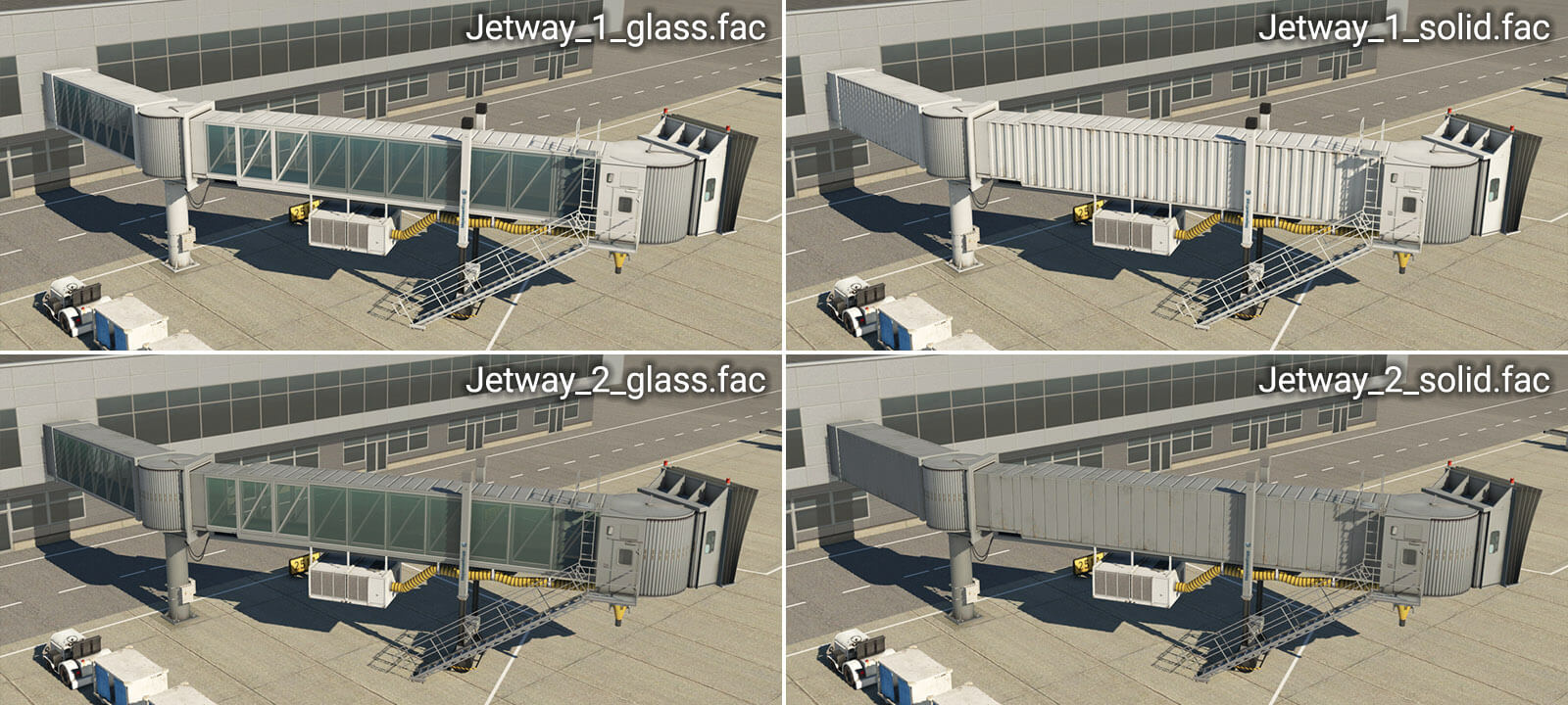
Jetway objects can be found in the WED library hierarchy at “lib/airport/Ramp_Equipment/Jetways“. Currently, four jetway-types are available:
Basic steps for the creation of jetways
1 – Pick the jetway facade and place the chain of nodes
2 – Set the “Pick Walls” checkbox
3 – Select the desired vertex (wall-type) for each segment
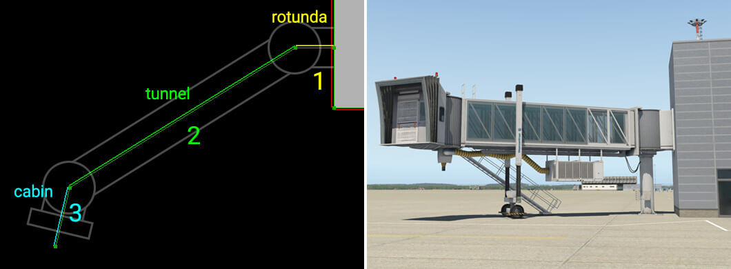
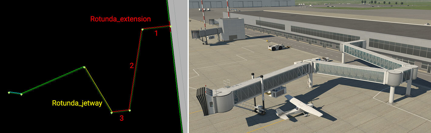
In a typical use case, the artist would place a chain with three segments (four nodes). Order of placement is important – always start at the terminal wall. (Note: Ctrl+Shift+R may be used to reverse the chain-order.) The artist must always set the vertex (wall type) manually. X-Plane can’t guess which segment is a telescopic tunnel and which is an extension or a cabin, for example.
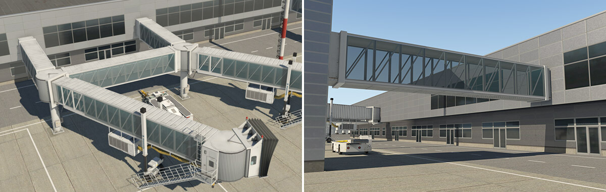
A typical jetway is always made of three parts. The first segment, rotunda, represents the connection between the terminal building and pivot point of the jetway bridge. The second segment represents the main body – a telescopic tunnel. The last segment must be the cabin.
Diagram illustrating the basic concept:
The parts of a jetway in detail
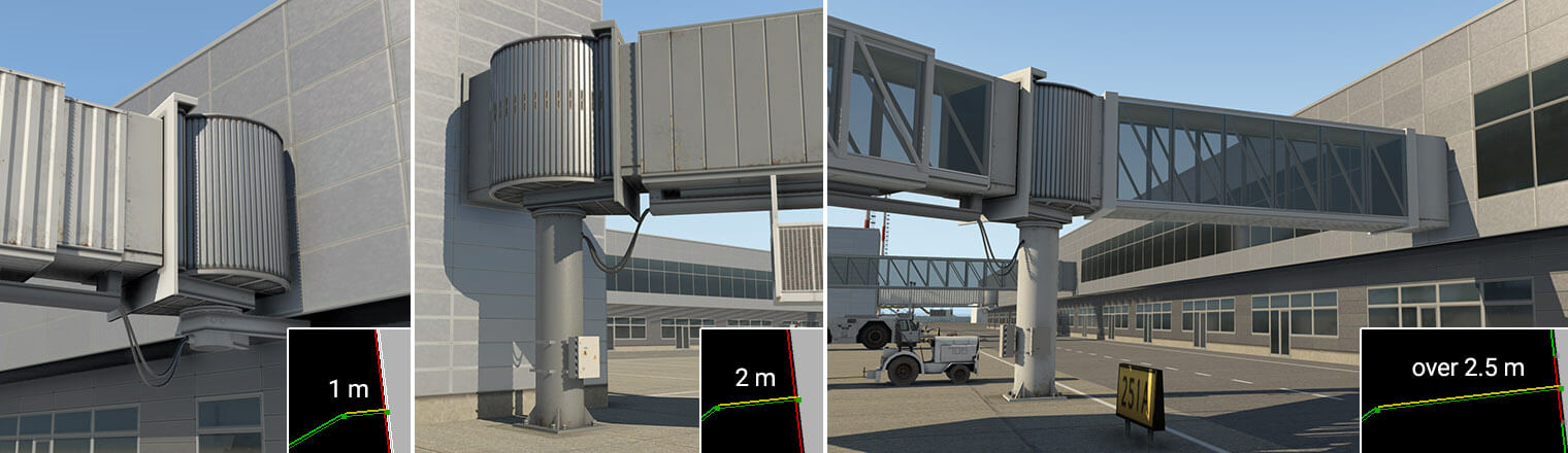
Segment 1 – Rotunda
The first segment (Rotunda) may be as long as required. However, the visual representation depends on its length. If it is very short (such as 1 meter), only a rotunda without a column appears on the wall of the terminal. If its length is between 1.5 and 2.5 meters, it shows the usual short neck and rotunda with a column, which is most common in the real world. With a length of more than 2.5 meters, and up to a maximum of 60 meters, it forms an extension bridge, ending with the rotunda and the column.
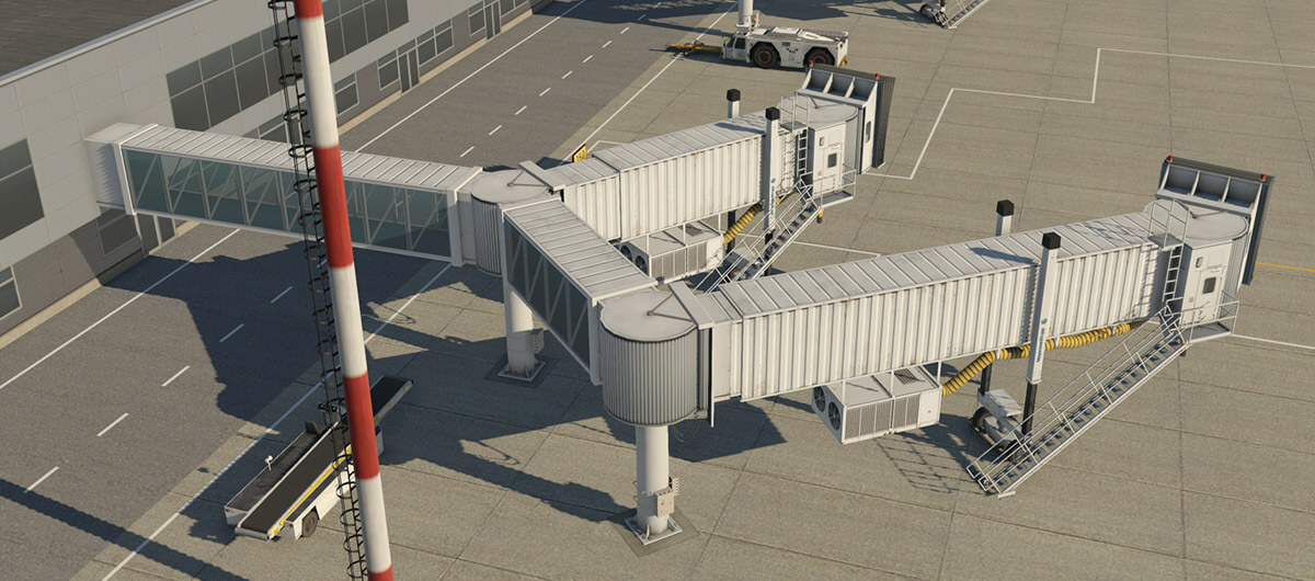
You may place multiple extension bridges in one chain to build very complex structures.
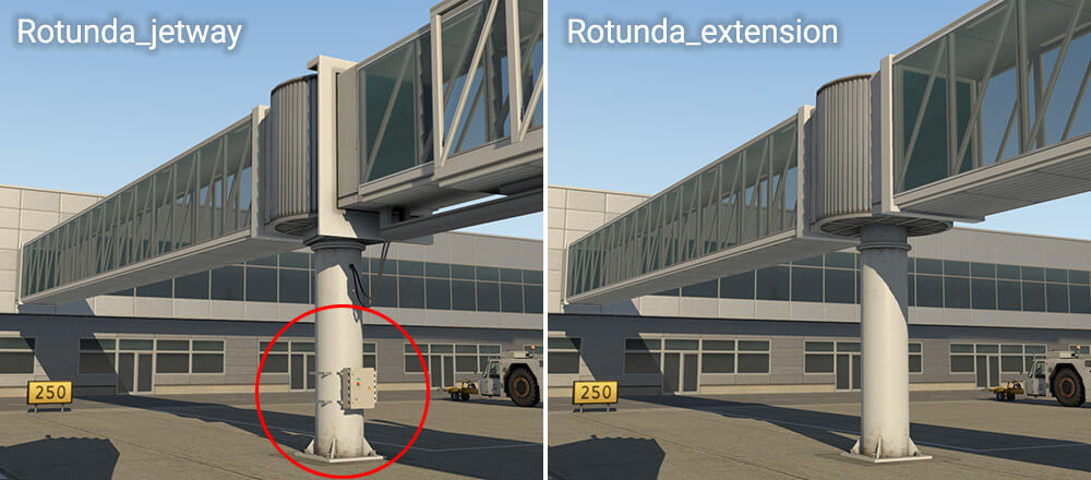
Rotunda segments have two vertex (wall-type) options – “Rotunda_extension” and “Rotunda_jetway“. Both behave exactly the same way, and the difference is merely visual. “Rotunda_jetway” has some electrical installation and is intended for use with telescopic tunnels, while “Rotunda_extension” is intended for additional extension segments.
Segment 2 – Tunnel
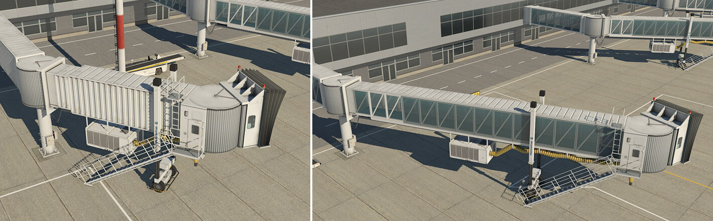
This segment must be at least 11 meters long and there are two options here. Artists may select the “Tunnel_parked” vertex (wall type) which is probably best solution for most situations. This automatically ensures proper selection of the telescopic bridge in retracted, or parked, positions. “Tunnel_parked” has some advantages for potential replacement with dynamic jetways at some point in future.
However you may also pick a specific length of tunnel, and construct it in an extended position. In this situation, the vertex name itself controls the extension range. For example, vertex “Tunnel_17-27.5m” would be suitable for lengths in the range of 17 to 27.5 meters.
Segment 3 – Cabin
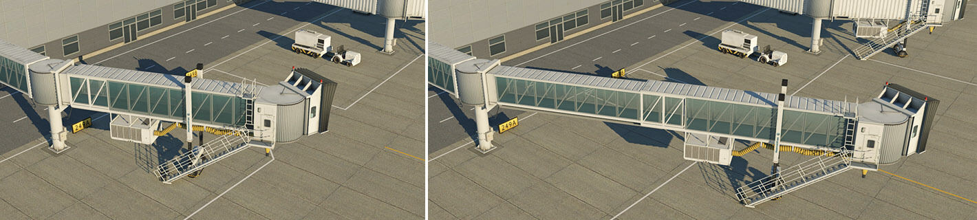
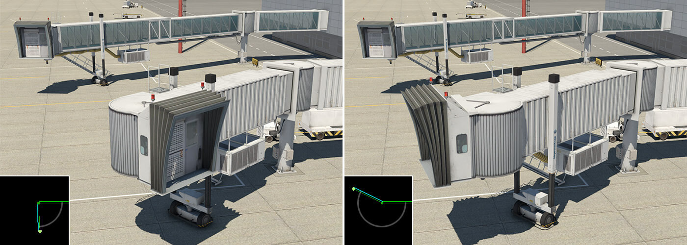
This is the final segment in a jetway chain. There is only one option for this segment – “Cabin“. The segment length isn’t important, but keep it in a reasonable range. The cabin object is always displayed at the beginning of the segment. The angle of rotation of the cabin should be approximately in the range illustrated below.
Special Segment – Connection
There is a special vertex (wall-type) named “Connection“. It works the same way as “Rotunda_..” but without the rotunda object itself. You can use this for connections between existing rotundas, or simply between buildings.
Useful hints
– Artists may combine different facades (white, gray, solid, and glass) to achieve, for example, a glass bridge with solid jetway tunnels.
– Glass versions of extension bridges sometimes have issues with transparency. Please DO NOT file a bug, as this is a known limitation of the rendering engine. There is no guarantee the correct draw order will be achieved from all view angles with all objects. Typically you may not see a neighboring extension bridge through a transparent extension. You will also not see a user-aircraft, or dynamic shadows.
FMOD Events are controlled by parameters – input variables that are sent into the FMOD sound engine by X-Plane. Besides the standard built-in FMOD parameters, X-Plane supports two other categories of parameters: cone parameters and DataRef parameters.
Cone Parameters
X-Plane supports two cone parameters:
xpevent_rel_heading (range is -180 to 180).

xpevent_rel_pitch (range is -90 to 90).
These parameters give the relative bearing of the listener to the event in the coordinate system of the event. The typical use would be to attenuate volume based on the relative bearing to form a sound cone.
An event’s orientation is inherited from the aircraft it is attached to, and modified by the Eulers (psi, theta, phi) in the .snd attachment file.
DataRef Parameters
X-Plane supports the use of any dataref (built-in or plugin-provided) as a parameter. Specific single indices of arrays can be accessed by appending “[0]” (or some other subscripting number) to the end of the dataref name, just like in OBJ animation.
FMOD events can also use wild-card sound parameters. These work by using [*] as the index to the dataref. When you do this, the event reads the index from the dataref that is specified in the .snd file via the PARAM_DREF_IDX directive.
The motivation for wild-card parameters is to re-use a very complex event (e.g. an engine sound) more than once, using the wild-card scheme to access different array indices for different sound instances. For example, in a twin engine aircraft you might use PARAM_DREF_IDX 0 for the left engine and PARAM_DREF_IDX 1 for the right engine, then use sim/flightmodel2/engine/XXXX[*] for your datarefs.
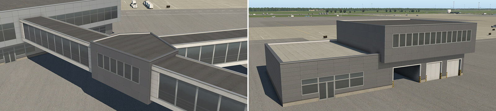
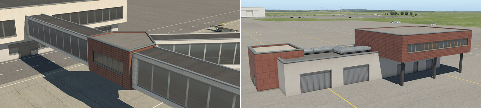
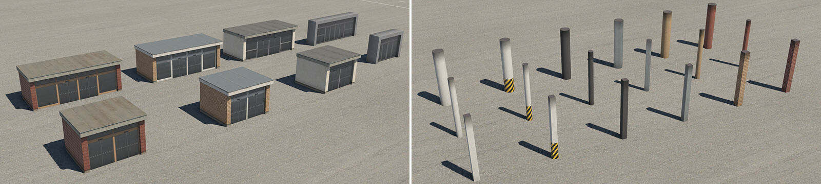
WED 1.6 in combination with X-Plane 11.10 or newer now includes an integrated ‘Terminal Kit’, comprising facades and supporting objects that are dedicated to the creation of modern airport terminals. This can be found in the WED library hierarchy at “lib/airport/Modern_Airports/Terminal_kit“. The Terminal Kit is entirely modular, with all parts designed to work together.
The basic concept is for the artist to utilize specific facades for corresponding parts of the building. For example, the kit features one facade for ground floor structures, and another for floors above. This approach asks a little more of the artist, because the facade footprint may need to be replicated multiple times, for each individual floor. However, this method offers far greater possibilities for the design of the structure. Windows, doors or gates may be placed exactly where the artist chooses, without this being restricted by the nature of the adjacent structure.
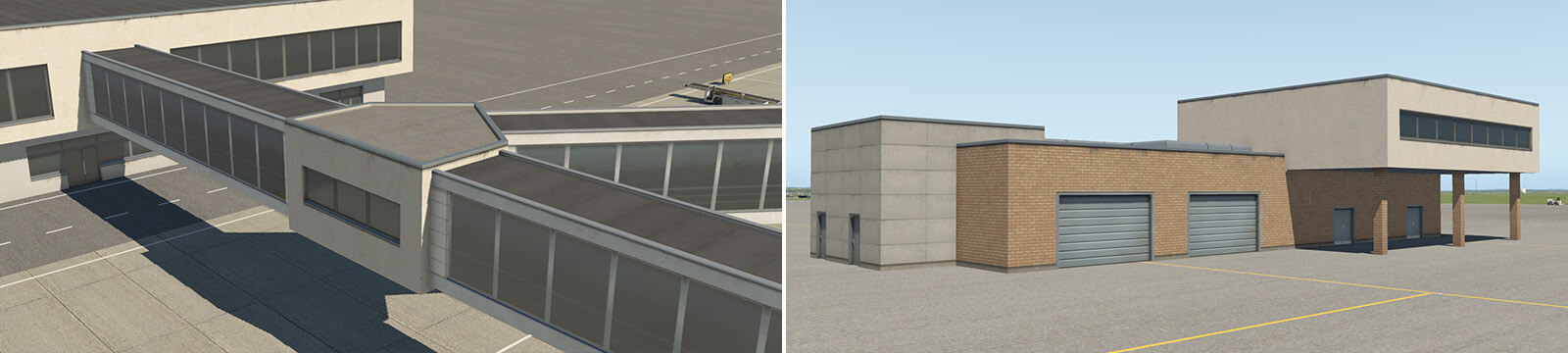
Key components of the Terminal Kit are prefixed with “term_” so these can be easily filtered in the WED library hierarchy. These are further divided into three logical groups:
The first group (term_building_..) is dedicated to the construction of the main building.
The second group (term_bridge_..) is dedicated to the construction of connecting bridges.
The third group (term_roof_..) is dedicated to the construction of the various roofing options.
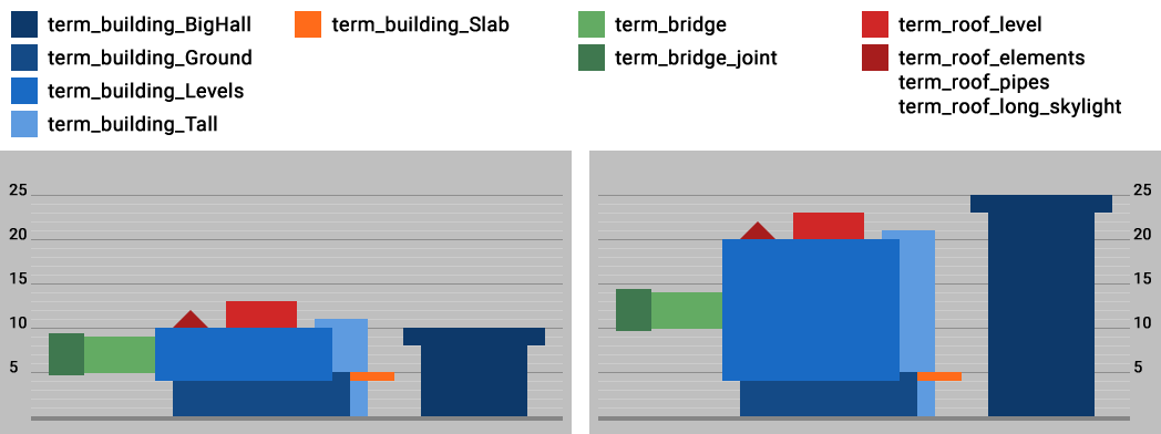
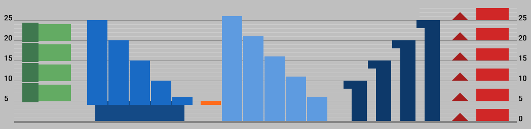
Most facades will comprise several floors, and as you can see, each floor must have an absolute height in units of 5 – namely 5, 10, 15, 20, or 25 meters (one exception is described later).
Diagram illustrating height and elevation options for Terminal Kit facade modules:
Note that roof elements are compatible with height levels (5, 10, 15, 20 and 25 meters). Artists may place them on”_Ground“, “_Levels“, “_Slab” and “_BigHall” modules. However, roof components may not be placed on “_Tall” modules.
Terminal Kit Components
term_building_…
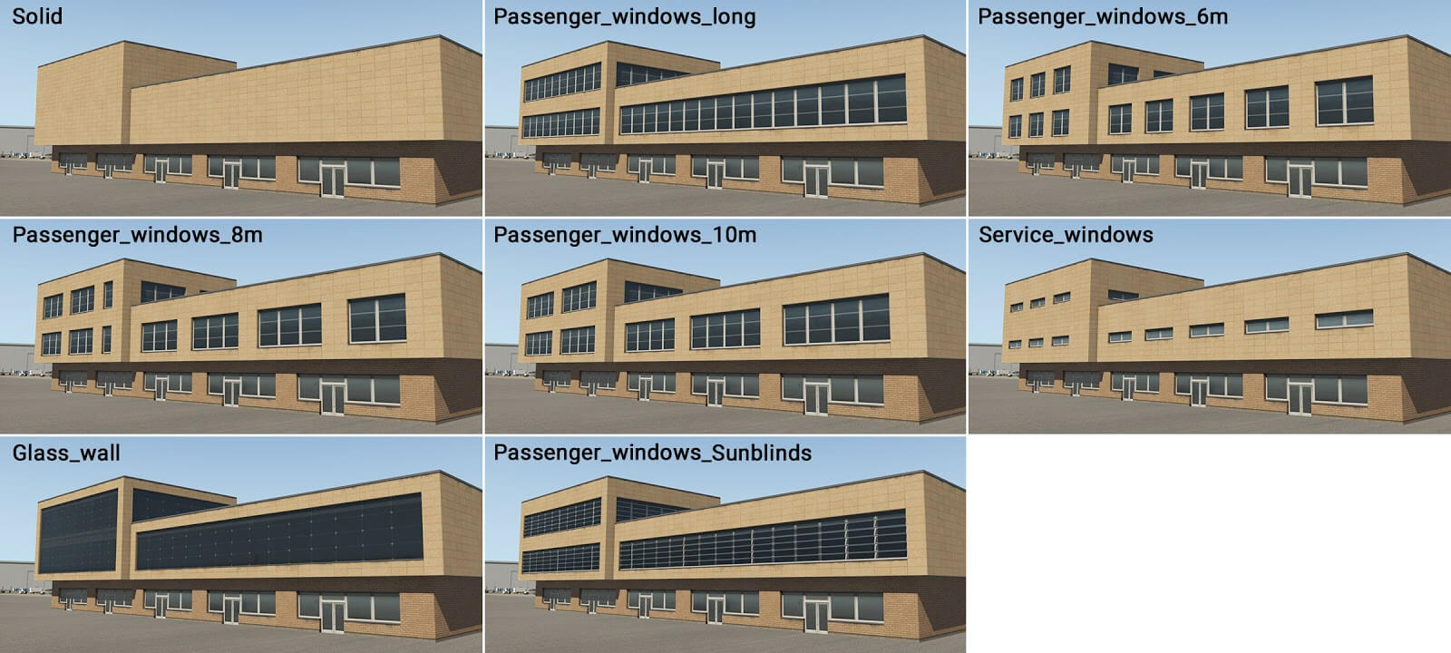
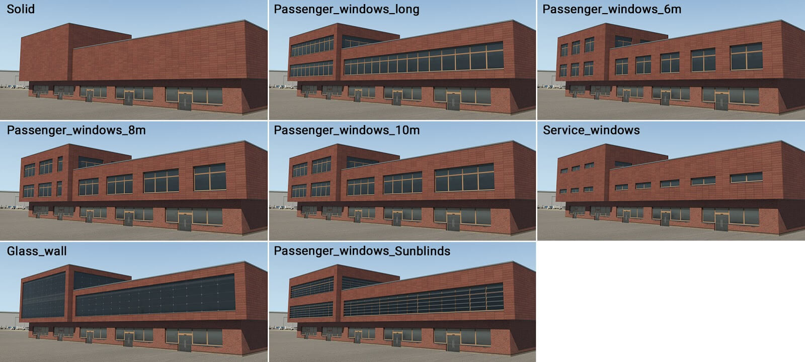
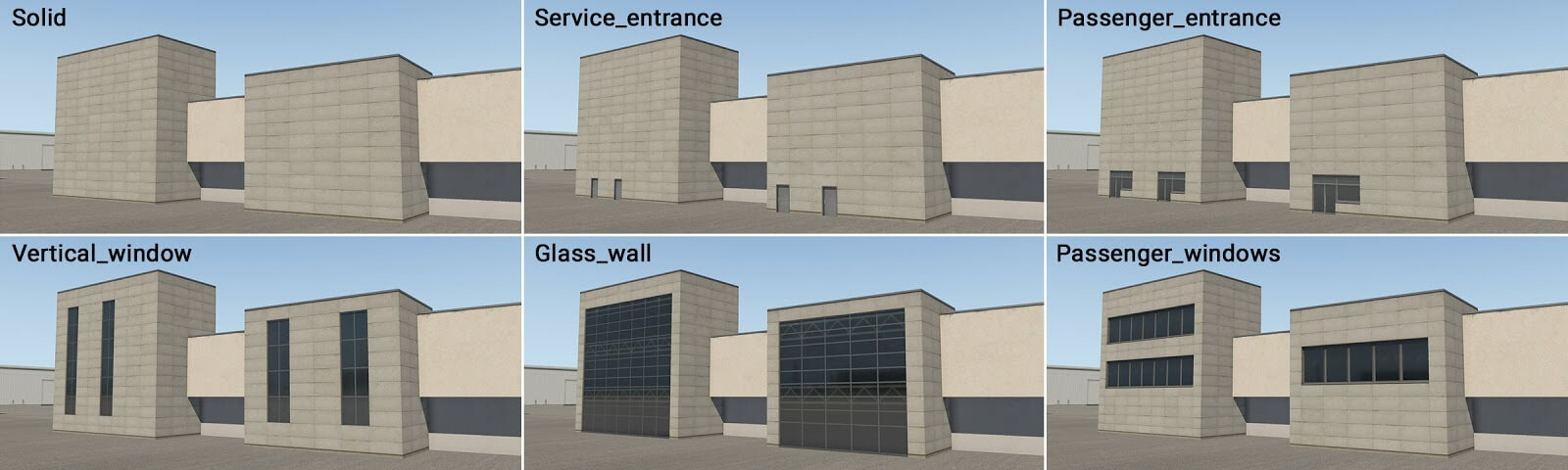
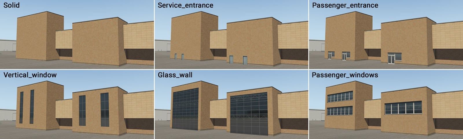
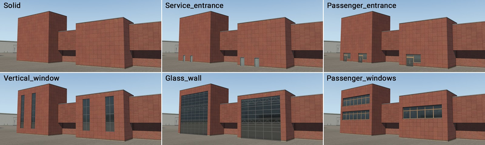
term_building_Ground_XX.fac
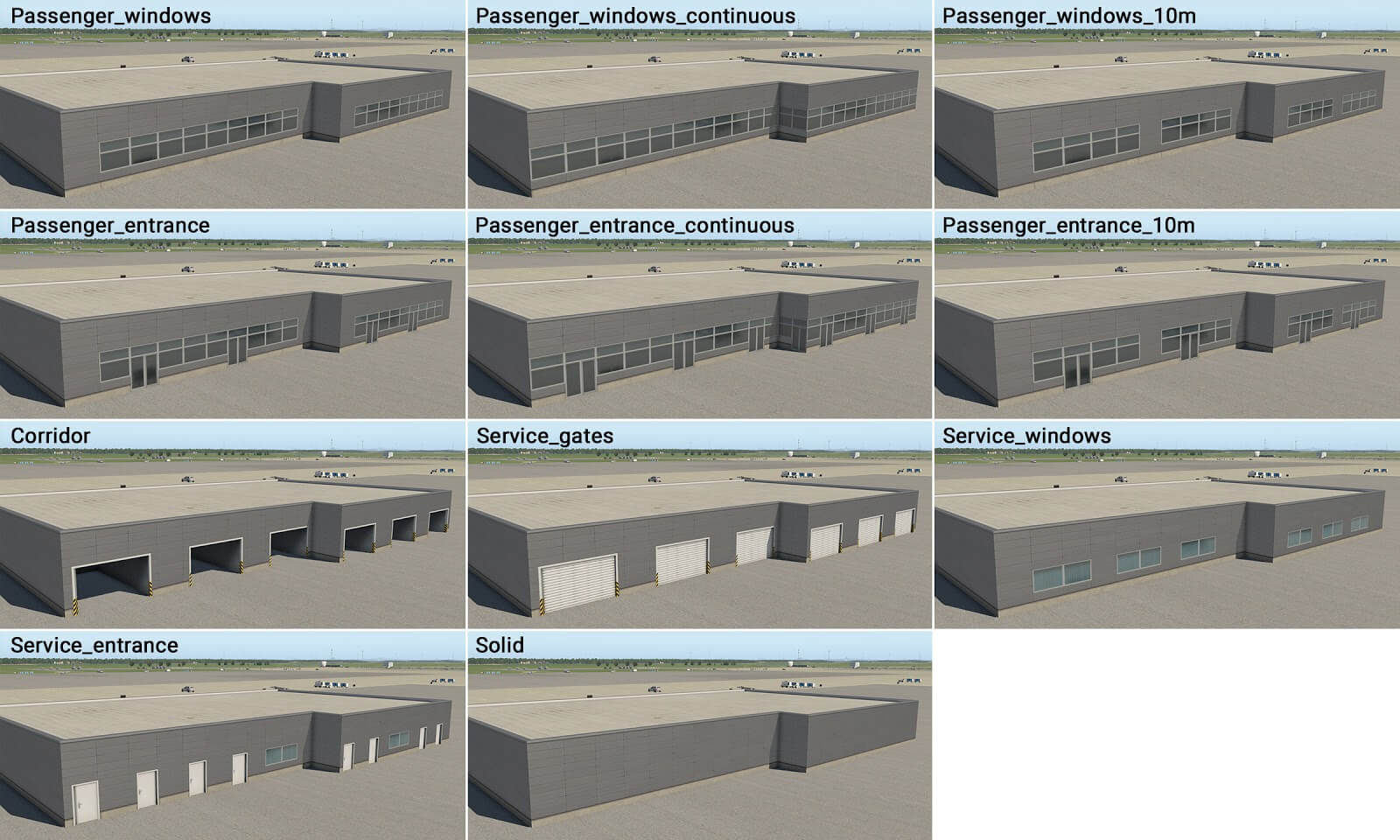
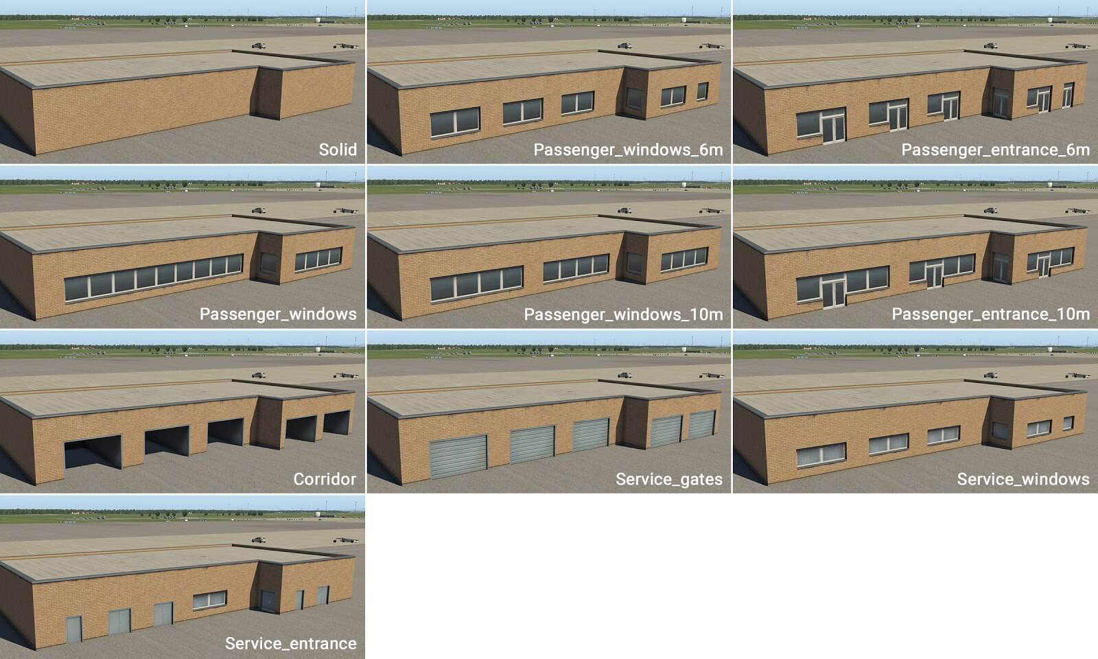
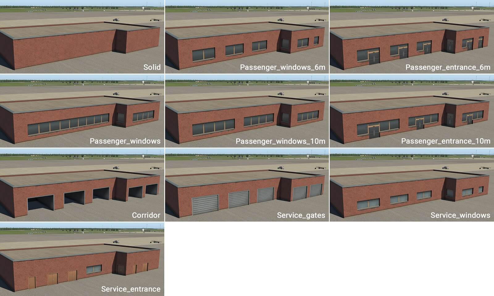
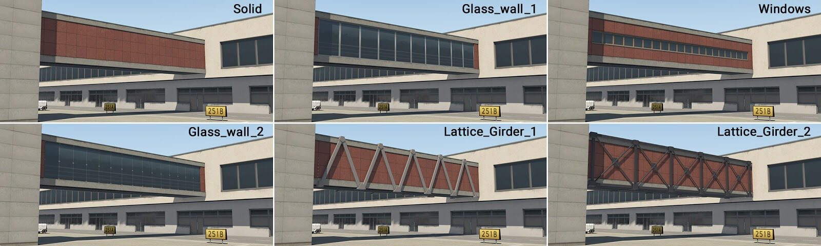
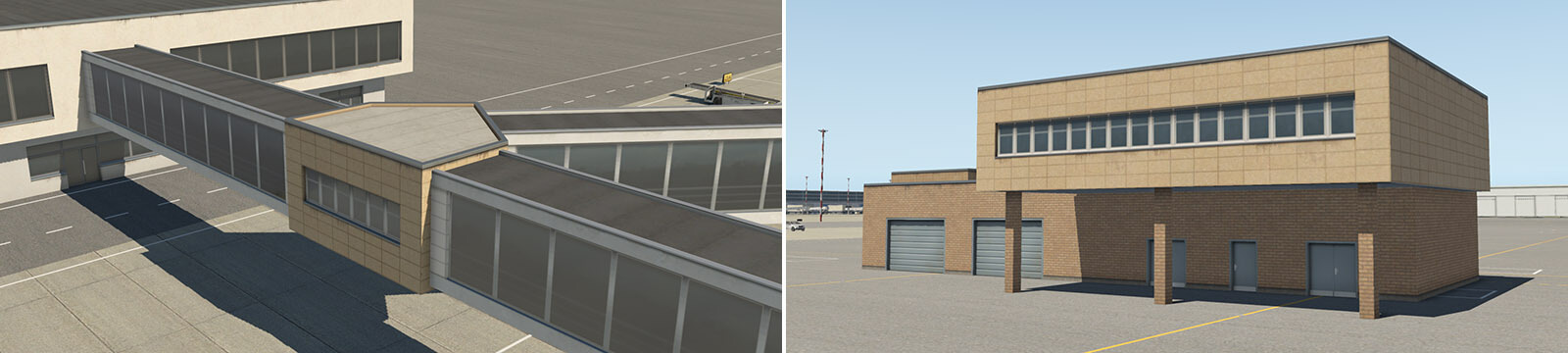
This is the first key component of a building. It has just one ground floor, and its purpose is to replicate the street level of a modern airport terminal. However it can also be used to create any single-floor building, and the artist may use it accordingly. This module has several wall-types–passenger windows, doors, service entrances and gates.
Sometimes three variants of passenger windows and entrances exist. This is a general principle which you will also find in other modules. The first variant (_windows) is designed for whole walls, meaning the facade comprises solid segments at both ends. However, sometimes the artist may require contiguous windows spanning the corners, and this is supported with the “_windows_continuous” variant. A third variant (_windows_XXm) is for long whole walls constructed in units of “XX” meters, with solid segments at either end. Any combination of these variants may be used together, to replicate the desired structure.
There are four stylistic variants in X-Plane 11.20 and newer:
term_building_Ground_01.fac
term_building_Ground_02.fac
term_building_Ground_03.fac
term_building_Ground_04.fac
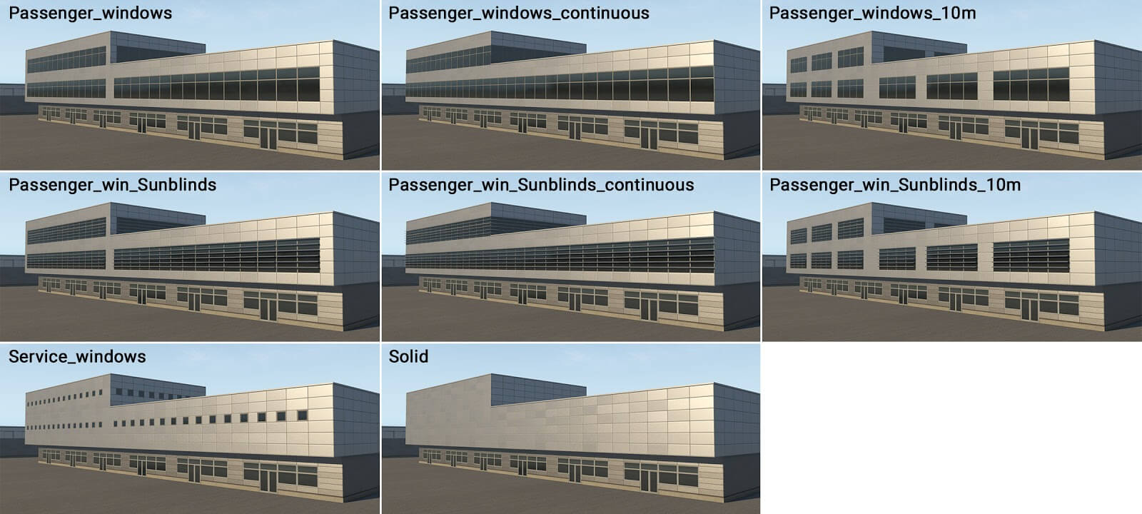
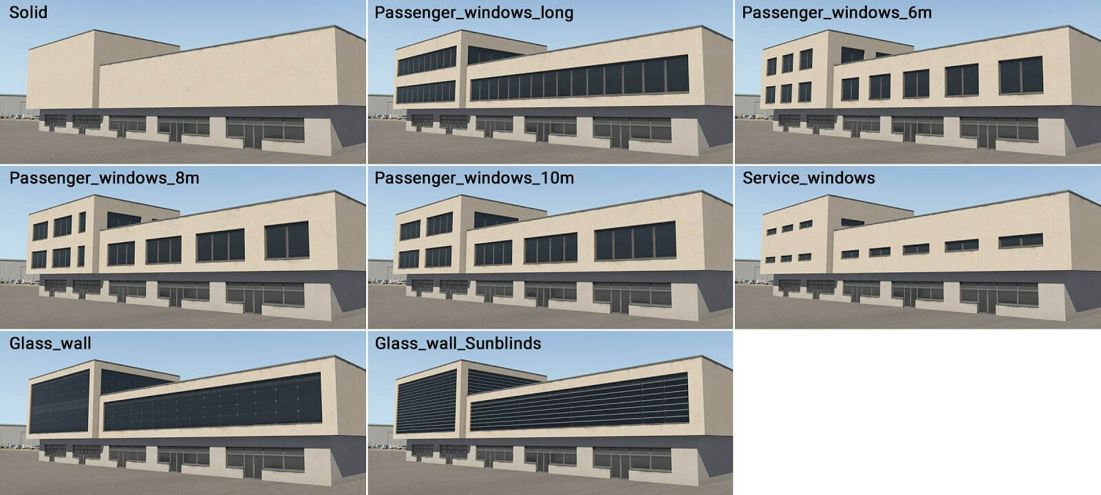
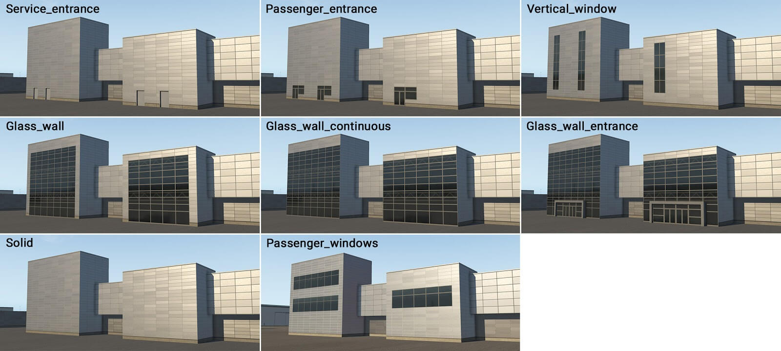
term_building_Levels_XX.fac
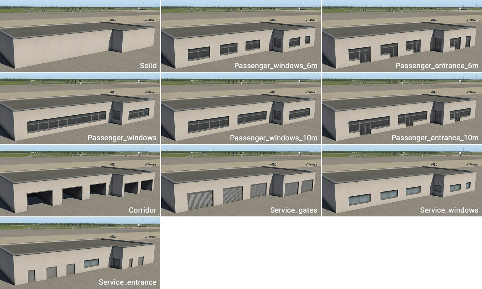
This is the second key component of a building. It is designed for (up to) three levels above ground. This module forms the “main” body of the terminal, and also has several types of walls (most of which have windows).
term_building_Levels_01.fac
term_building_Levels_02.fac
term_building_Levels_03.fac
term_building_Levels_04.fac
This module also has one very specific usage: When the height is set at 5 meters above ground-level, this component is rendered as a ‘slab’ (no matter which wall type is selected). This can act as a flat roof, and may be used above the ground floor, or with columns (described later). However in this case it is technically higher than a normal floor (6 meters) so artists may not place roof elements on it. Here is an example:
term_building_Tall_XX.fac
This module has various purposes: volume extensions, stair-towers and other vertical parts. It is slightly higher (by units of 1 meter) than adjacent modules, and can be inserted into other basic modules, or used as a stand-alone module.
term_building_Tall_01.fac
term_building_Tall_02.fac
term_building_Tall_03.fac
term_building_Tall_04.fac
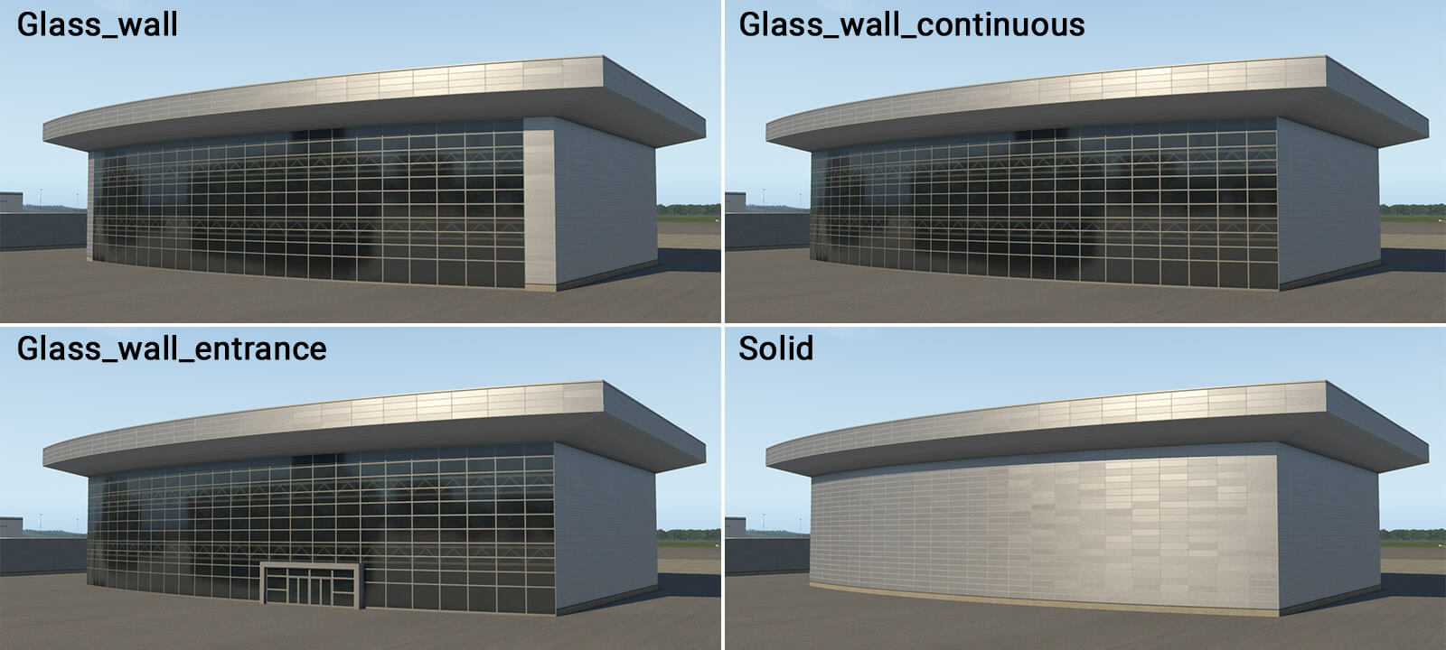
term_building_BigHall_01.fac
This is special module for the creation of large halls with glass walls. It is intended for simple shapes like rectangles, and can’t handle negative corners (concave angles).
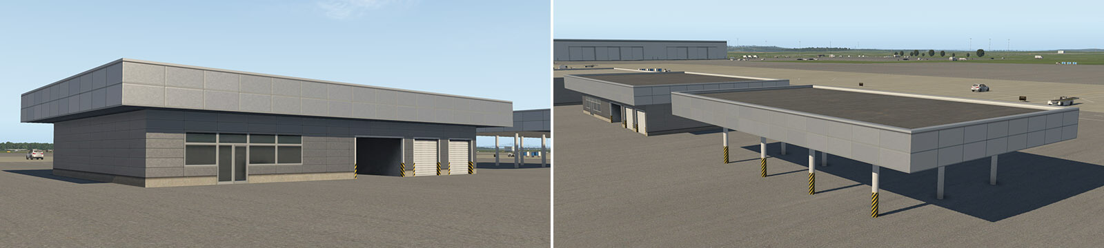
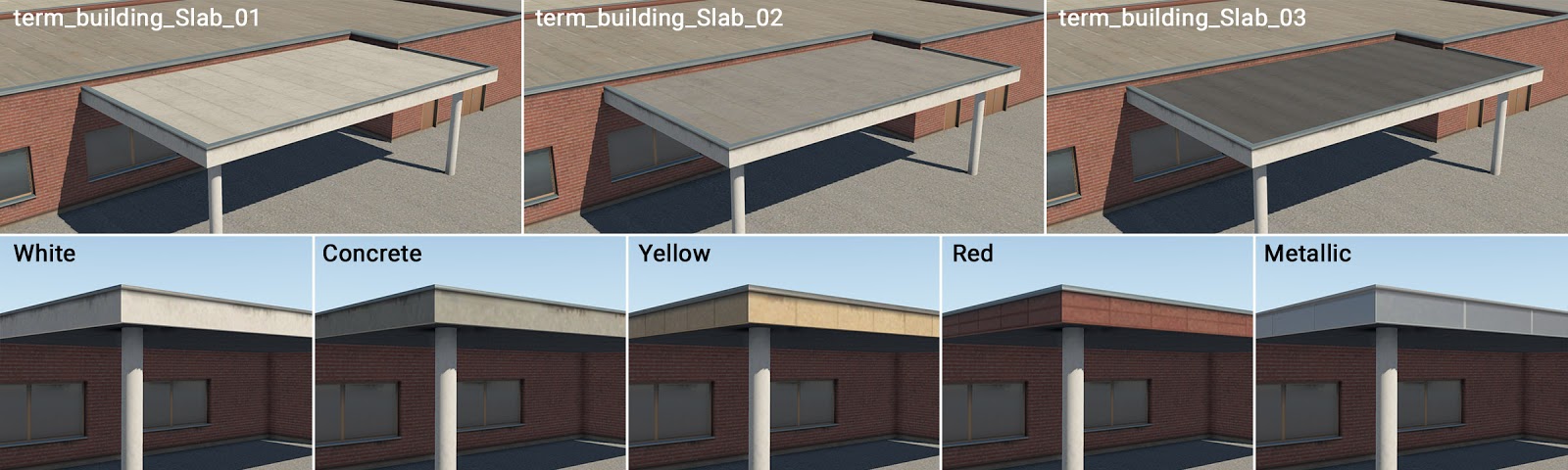
term_building_Slab_01-03.fac
This is another special module for the creation of simple slabs. It is available in three different roof colors, each with five edge-material options. It is also compatible with all roof elements, just like “_Ground” module.
term_bridge_…
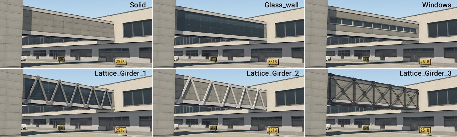
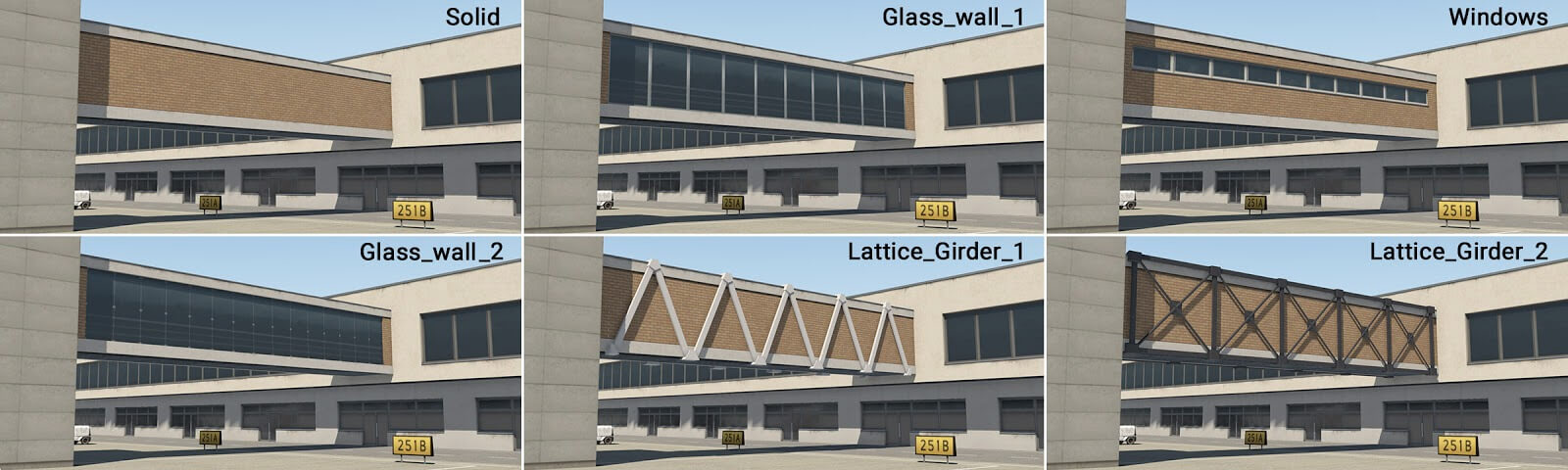
term_bridge_XX.fac
This module is used to create bridges. Technically it is similar in construction to the “_Levels” module, but makes only a single floor. If the artist needs two bridges above each other, this is achieved by duplicating the structure at different heights above ground.
term_bridge_01.fac
term_bridge_02.fac
term_bridge_03.fac
term_bridge_04.fac
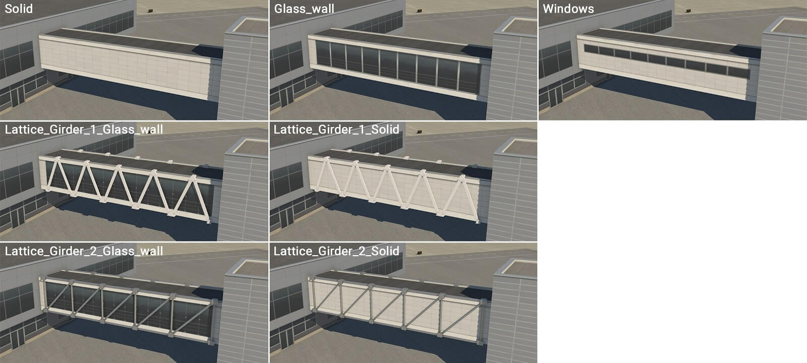
term_bridge_joint_XX.fac
This module is similar to term_bridge_XX.fac, but with a more substantial appearance, supporting just two wall-types – solid, and (very simple) windows. The main usage will likely be situations where two bridge sections are joined together. However, this module may also be used as a second floor, above a ground floor structure.
term_bridge_joint_01.fac
term_bridge_joint_02.fac
term_bridge_joint_03.fac
term_bridge_joint_04.fac
term_roof_…
term_roof_level_XX.fac
This module provides for the creation of roof-superstructures. The module is 3 meters in height, and this is the exception mentioned earlier. The absolute height of this facade must therefore be 8, 13, 18, 23 or 28 meters (as opposed to 5, 10, 15, 20 and 25 meters).
term_roof_Level_01.fac
term_roof_Level_02.fac
term_roof_Level_03.fac
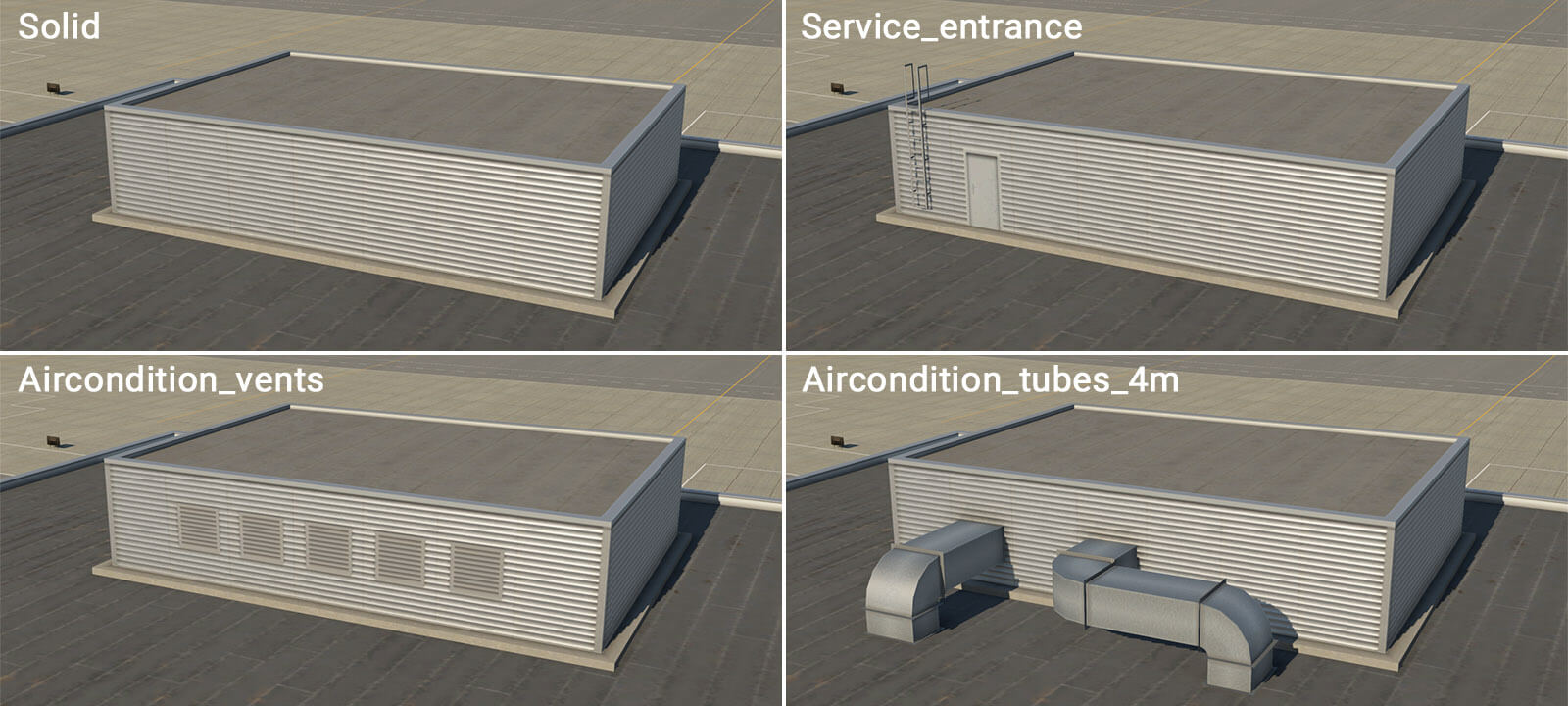
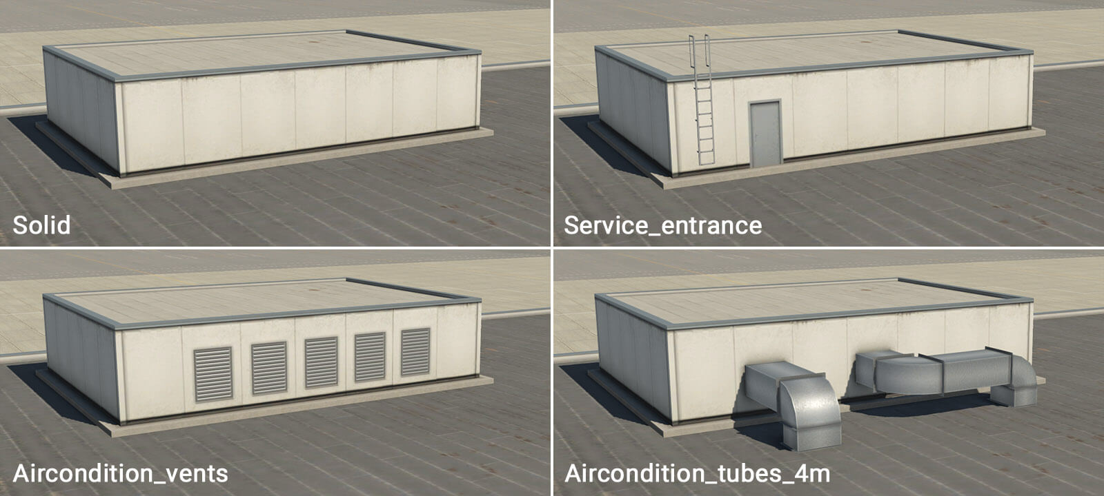
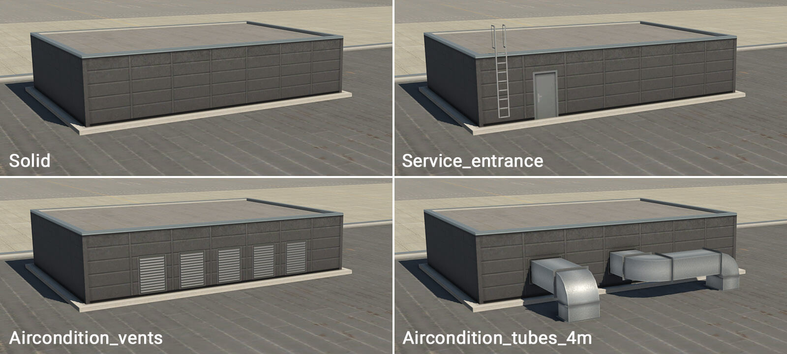
term_roof_elements_01.fac
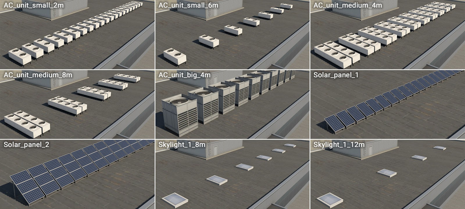
This is very special module. Technically it has invisible walls and roof, and therefore only the attached objects are visible. This module may be used to support various roof elements, like air conditioners, solar panels or small skylights. This module’s facade isn’t ‘closed’, so artists will see a chain of linear-segments in WED. Attached objects are placed at the center of these line-segments.
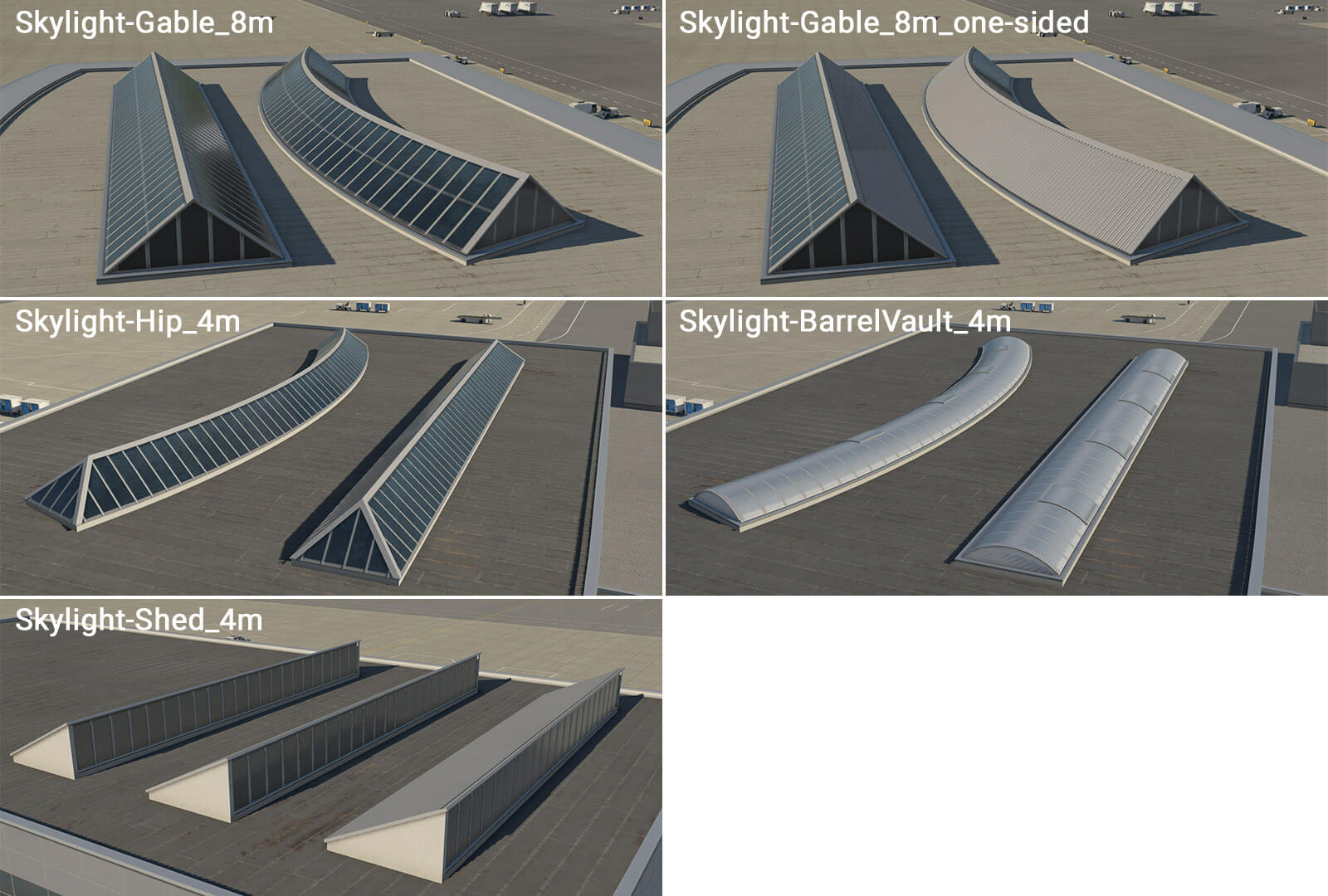
term_roof_long_skylight_01.fac
This is another specific module that forms various longitudinal skylights. This behaves like other WED linear-features, with the line (or chain of lines) itself representing the axis of the skylight.
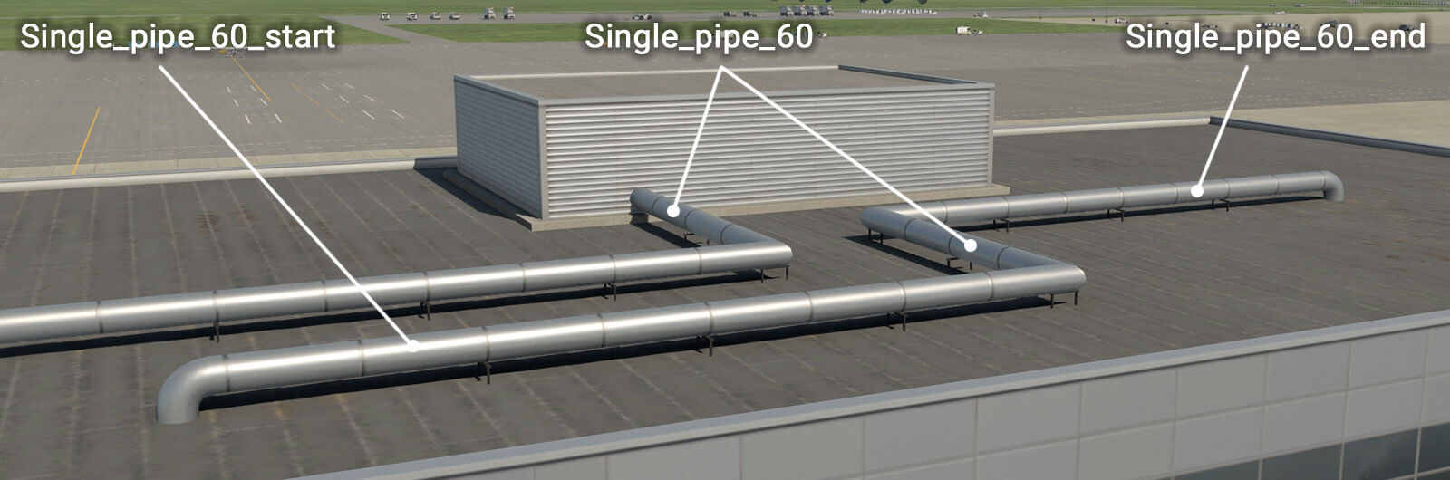
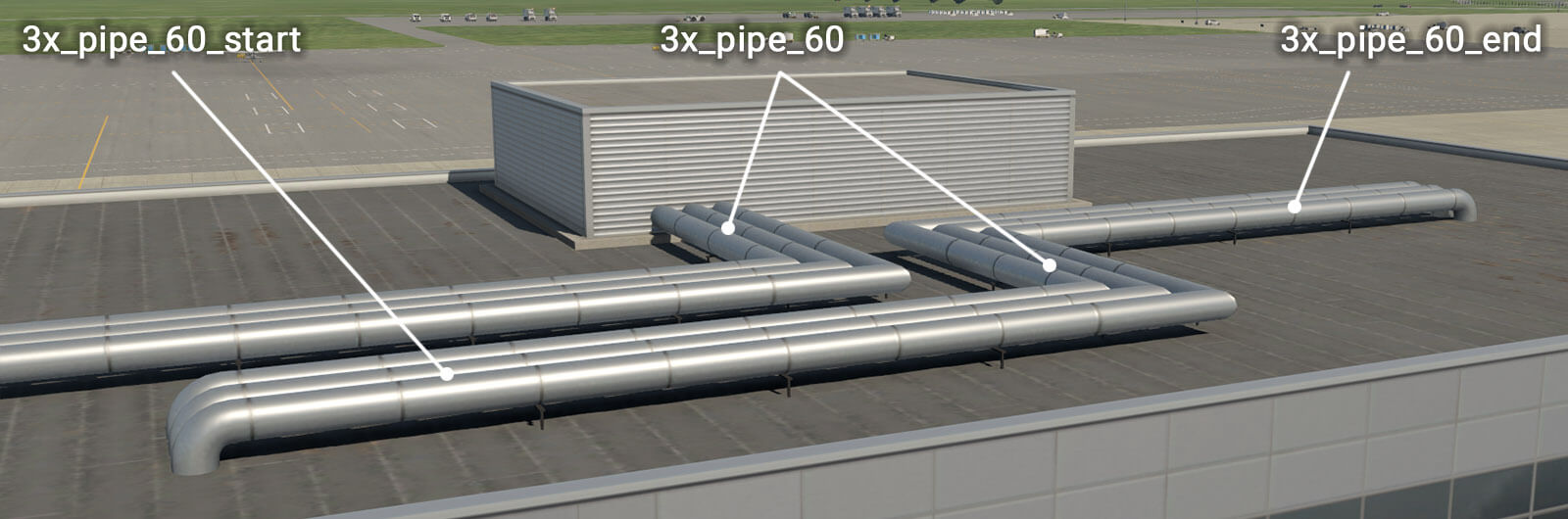
term_roof_pipes_01.fac
The same principle applies here as to the skylights module, except this module is not limited by one segment. The artist may draw any number of segments in a chain. The basic facade wall generates horizontal pipes which can be connected to another module, such as “_roof_level“. However, there are also special walls with a “_start” prefix, and “_end” suffix. This is useful when pipes project vertically from a roof. The direction of the polygonal chain in WED is important here, and this is why the artist must define start and end segments for the facade.
Other objects
There are other useful objects that can be placed manually:
Entrances
Some facades already have walls called “_entrance” but sometimes it will be useful to place them manually. Moreover entrances are generic, and can be used with various facades as needed.
Columns
Additional important objects are columns, and separate ground-floor and upper-floor columns are available. Columns are placed manually where required, to form a plausible structure. Columns are available in two lengths – 4 and 9 meters. Shorter columns may be used under “term_building_Levels” facade and under “term_bridge” and “term_bridge_joint” modules (with a height of 10 meters at the lowest position). Higher columns can be used under bridges or joints (with a height of 15 meters at the lowest position).
Useful hints
-This Terminal Facade kit comprises basic modules of 2-meters in horizontal length. This means that a single metal panel is two meters long. There is no explicit reason to be aware of this, except that it may prove useful when positioning manually placed assets (eg entrances and columns) adjacent to the terminal modules themselves.
-All roof textures have some kind of directionality (appearing as ‘strips’). This is always perpendicular to the FIRST segment of the polygon (the white line in WED). You can rotate segments in WED by pressing Ctrl+R. This is important (especially with bridges) whereby the first segment should be oriented in the direction of the bridge axis.
-Large terminal buildings often have a very complex footprint. Don’t attempt to replicate this complex shape with just a single facade polygon. It’s much better to divide the structure into smaller logical shapes. This also helps when dealing with roof directionality, and where there are large differences in terrain elevation at the extreme ends of the building.
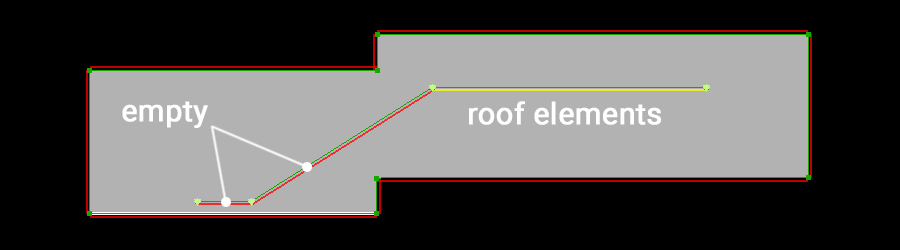
-At times, the terrain may have a significant gradient. This may cause roof elements to ‘float’ above the module below, or sink into it. This is because modules are rendered at the exact height of the center of the first polygon segment. To control for this, some roof modules have an “empty” wall. The artist may start the module chain with an “empty” segment, near the center of the first segment of the underlying module. The artist then draws the second empty segment in the desired location of the (visible) roof element, and this should render at the correct height.
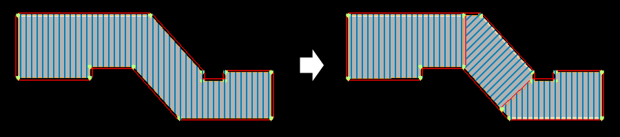
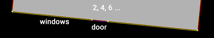
-When an artist requires doors, gates or corridors at exact locations in a long module wall, this may be accomplished by the insertion of a node, and a change in wall-type (even in straight segments). Keep in mind that basic modules are 2 meters in length, so try to use segments that are approximately 2, 4, 6 or 8 meters long. This helps avoid unwanted stretching.
-The height of one metal panel isn’t technically one meter, but actually 96 centimeters. The reason for this is related to jetways, but not important to artists when constructing the terminal modules. Likewise, the exact height of floors are actually 4.6 m, 9.4 m, 14.2 m, 19 m and 23.8 m.
The X-Plane 11 particle system follows a fairly standard game-industry design:
A particle system consists of a collection of emitters and particles. There can be many particle systems running in X-Plane at the same time, and they do not interact with each other.
A particle system’s behavior is controlled by a particle system definition text file. More than one particle system can use the same definition file at a time.
Particle Types
Every particle in a particle system has a type, and the definition file defines the behavior of every particle type. Typically you will have a small number of types per definition file. For example, a definition file that contains “smoke and fire effects” might contain three types of particles: a flame particle, a white smoke particle, and a black smoke particle.
The particle type definition controls the appearance and behavior of the particle over time, including what textures it uses and how it grows/shrinks and fades over time.
Every particle that is created in a particle system has a finite lifetime (measured in seconds) before it disappears. The particle definition file defines how the particle type is drawn over that lifetime. For example, a typical behavior is to make the opacity of the particle fade from 100% to 0% over the lifetime of the particle, so that the particle slowly disappears.
All properties of the particle type that can be key-framed are key-framed over either the lifetime of that particle, or by data-refs. You can use more than one key-frame table; the results of each table are multiplied to get the final result.
Emitter Types
An emitter creates particles; every emitter has a type, and the emitter type definition defines how the emitter creates particles.
The emitter always creates the same type of particles, but it can control the particle’s initial properties, including its initial size, its initial opacity, and how long it lives for.
Emitters are used in the simulator by attaching them to objects or aircraft. The emitter would be attached at a particular location on an OBJect with a particular direction; if the object is on an airplane, the emitter moves with the airplane. For example, you might put an emitter of smoke puffs on the exhaust pipe of an aircraft.
For convenience, X-Plane lets you put one or more sub-emitter into each emitter. Each sub-emitter can emit its own type of particles with its own properties. The motivation here is to make it easy to attach a lot of emitters to a single point in an object.
For example, our gun-barrel emitter contains two sub-emitters: one for the muzzle flash (emitting a small number of fire particles) and one for the smoke (emitting a larger number of smoke particles). By wrapping both sub-emitters in a single emitter, it’s simple to attach the one “gun barrel” emitter to the tip of a gun barrel on a fighter.
The various properties of the emitter (number of particles created per second, initial velocity, etc.) are key-framed based on datarefs. So you can specify that an emitter makes more particles (or faster particles, or bigger particles) as the engine’s N1 spools up. In this way, an emitter can dynamically change its stream of created particles based on inputs from X-Plane.
Datarefs attached to emitters can use wild-cards for array indices. When you specify [*] for a dataref index (e.g. sim/flightmodel2/engines/N1_percent[*]) the * is replaced with an index number that comes from the OBJ file where the emitter is attached. This lets you use a single ‘generic’ emitter for all engines in your aircraft and specify the engine index number each time you use the emitter. (This mechanism works the same as wild card parameters in FMOD.)
Many parameters of the emitter type definition can be randomized. In this case the parameter ha a lower and upper bound that can be edited separately. Since the parameter is key-framed, the amount of randomization (the distance between the two parameters) can vary based on a dataref.
Effect Types
Emitters are attached to parts of the X-Plane world (scenery objects, airplane objects, etc) and run continuously based on their volume. This is good for continuous sources of particles like a smoke stack, but it is not good for a finite event, like an explosion.
An effect is a collected sequence of key-framed emitter locations and values. An effect is something that happens over a time and start location. For example, an explosion effect might contain instructions to run a fire emitter for 10 seconds.
The properties of an effect are key-framed to the time of the effect; the effect has a finite total duration. Thus for an effect you can create a smoke emitter that creates a lot of smoke and then have the smoke level slowly die down.
Effects cannot be attached to objects; rather X-Plane uses effects directly at specific times, e.g. when a bomb hits the ground or when the airplane crashes.
Accessing the Particle System in X-Plane
As of X-Plane 11.30d2, the X-Plane B737 has been updated to use the particle system and can be used as a reference.
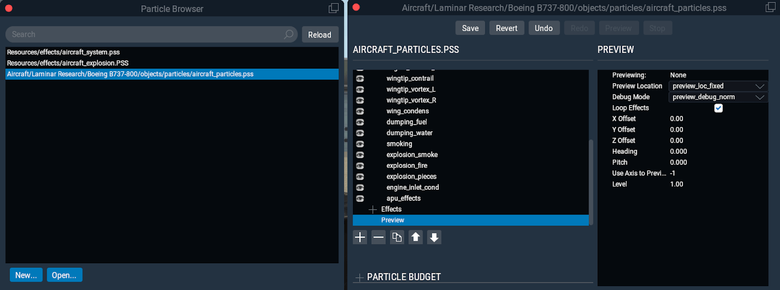
Pick “Show Particle System Browser” from the developer menu to access the in-sim particle system UI. You will see a list of all currently loaded particle system definition files (.pss files). You can edit any loaded particle system shown in the browser by double-clicking to open its editor. Note that these windows can be resized or popped out, and the width of the columns in the .pss window can be adjusted.
To create a new particle system, click the “New…” button and pick a particle system file on disk. The location of your particle system on disk matters because only textures in the same folder as the particle system (or in sub-folders) can be used.
To open and edit a particle system not currently in use by X-Plane, click the Open… button and browse to your .pss file.
The particle system editor
The upper left column (named for whichever particle you double clicked to open from the browser) is a hierarchy list of all particles, emitters, effects etc. + preview and texture tab. This may be hidden if the Particle Budget column is expanded. Click an item to view its properties; icons under this section are: create, delete, duplicate, move up, move down. The eyeball icon next to the various emitters lets you disable emitters globally.
The lower left column is the particle budget. For the PREVIEW only, this shows how many particles of each type are being used, which lets you figure out if you have enough particles of each type budgeted in the system. Note that particle systems used in the sim and not in the editor preview are NOT shown, so sadly you cannot use this to debug budget problems in the live sim.
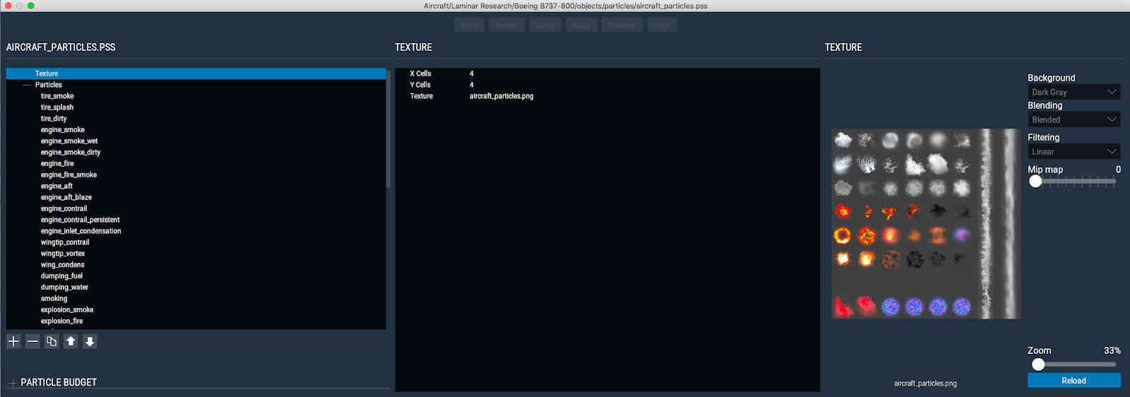
When “texture” is selected from the hierarchy, the texture preview appears on the right side.
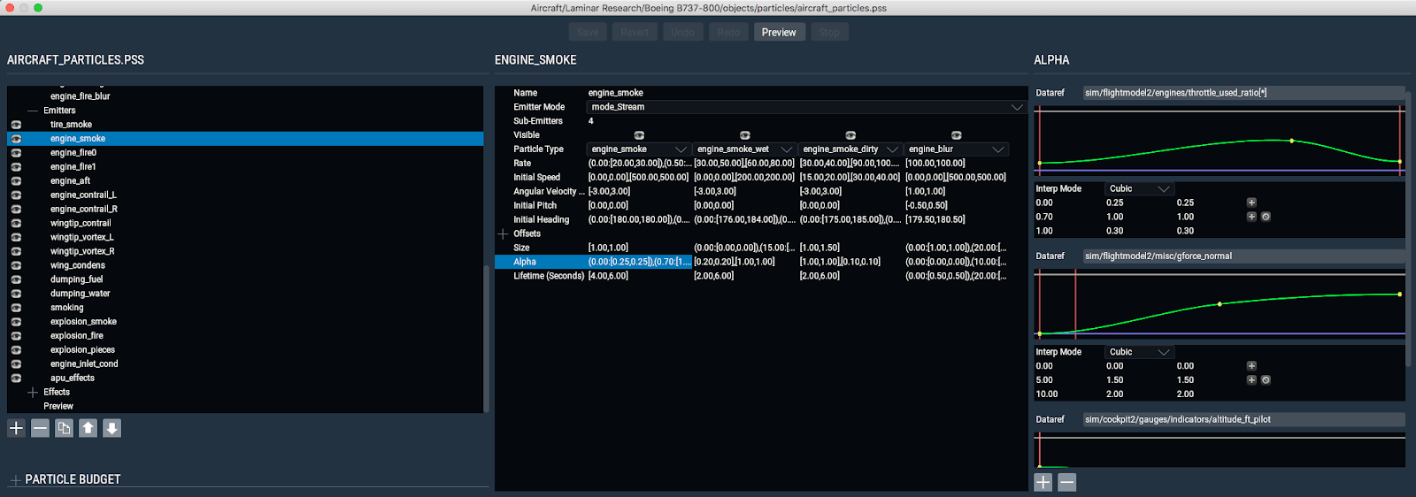
The middle section is the property editor and is named for whatever is selected in the hierarchy. When an emitter is selected, the sub-emitters form multiple columns.
When a property that can be key-framed is selected in the middle view, the key frame editor appears on the right side. The add/delete buttons on the right let you add a second key frame table or delete the bottom one.
Each key frame table lets you pick a dataref or other key frame source, and then edit the key frame table either graphically by dragging nodes or by clicking. Option-click on a key-frame curve to add nodes graphically, or use the + (add) and ø (delete) icons on the right.
The key-frame interpolation mode popup changes the algorithm by which the key frame points are attached.
If the key frame property contains more than one value (E.g. two for a randomized value between two bounds or 3 for RGB colors) you can drag each line independently.
Top buttons provide access to: save/revert the .pss file, undo/redo edits, and preview/stop previewing the selected emitter or effect. (You cannot preview a particle type directly – you must preview an emitter that emits them.)
Particle Properties
These settings affect all particles of a given type. Some properties can be key-framed either by a dataref or by “particle lifetime”, which makes a property change over the life of each particle. When “particle lifetime” is used, the key frame table runs at different speeds for long-living and short-living particles.
Name: this is the name you see in the hierarchy – X-Plane ignores it.
Max particles: this is the maximum number of particles of this type you can have at once. The biggest you can set this is 16384. Set this large enough that the system does not run out of capacity, but smaller is better.
Physics Properties
Gravity: this is how heavily gravity makes the particles fall. Negative numbers make them rise. A value of zero means no gravity.
Drag: this is how fast the particles slow from their initial speed to the speed of the outside air – higher numbers give more drag. A value of zero means no drag.
Angular Velocity: this is how fast the particle billboard spins over the life of the particle.
Turbulence: this is how much each particle is randomly bounced around by turbulent air.
Collision Mode: this defines what happens when the particle hits the ground.
None: the particle is not checked against the ground. This is the fastest for CPU – use this if you do not need to collision test.
Bounce: the particle bounces off the ground. Set Elasticity to make the particle bounce more or less.
Die: the particle disappears when it hits the ground.
Rendering Properties
Billboard Mode: this controls how the particle is drawn in 3-d.
Billboard – the particle is a square and always faces the camera – good for smoke.
Axial Billboard – the particle is a long rectangle, spinning around the direction it moves – possibly good for gun fire.
Ribbon – the particle is a long connected chain of quads with the texture repeating – good for contrails that must be very long.
Blending Mode: this controls how the alpha of the particle is combined with the scene.
Normal – the particle blends over the background, like a photoshop layer – good for smoke.
Additive – the particle adds light – good for lights and explosions. Similar to how the OBJ lights work.
Pre-multiplied – the particle is applied using “pre-multiplied” alpha – areas with opaque alpha act like ‘normal’ and areas with clear alpha act like ‘additive’. Your particle’s RGB must be drawn over a black background.
X/Y Grid Divisions: this defines the grid of texture cells for this particle. Each particle can use its own grid so that some particles can be big and some small.
Start Cell/Cell Count: this defines the list of cells that animate to draw the particle. The upper left cell is 0, and then they increase from left to right, then down, like a book.
Repeat: how many times the cell sequence repeats over the life of the particle.
Randomize: if checked, each particle gets a random texture cell and does not animate.
Animation Rate: this lets you customize the speed of the cell animation over the life of the particle.
Scale: this controls the size of the particle – it can grow or shrink over time.
Alpha: this controls how opaque the particle is – you can fade it out over time.
Length: for axial billboards only, this is how long the particle is (separate from the width).
Ambient, Diffuse: this controls how much the particle is lightened by the lighting conditions of the world.
Emissive: this is how much the particle creates its own light, so it is visible at night.
Tint: this is an RGB control that can ‘tint’ the color of the billboard if needed.
Emitter Properties
Each emitter contains one or more sub-emitters – the idea is to allow several emitters at a single spot (e.g. smoke and fire for a rocket) by attaching only one emitter in an OBJ.
Name: this is the name you see in the hierarchy – this is used to specify the emitter in the OBJ file.
Emitter Mode: this controls how particles are emitted.
Stream: particles come out continuously over time. This is the default mode and is useful for smoke. You must use streaming mode for ribbons.
Burst: a large number of particles are all emitted at once. This is used only for effects, and not for emitters attached to objects.
Attach: a single particle is kept attached to the emitter at all times. This can be used to create a single ‘flame’ billboard on the end of an engine, for example.
Number of sub-emitters: change this to add and remove sub-emitters.
Sub-Emitter Properties
Visible: you can temporarily hide an emitter to remove its particles from the particle system preview. This is used only for authoring, and is not used in the final particle system.
Particle type: this selects which particle type the emitter emits.
Rate: this controls how many particles are emitted per second.
Initial speed: this is how fast the particles are moving when emitted. This speed is relative to the speed of the OBJ they are attached to (e.g. the airplane).
Angular Velocity Multiplier: this scales the rotation from the particle definition itself.
Initial Pitch/Initial Heading: this controls the direction the particle flies relative to the attached object. An emitter on an OBJ that is not animated (in the OBJ) and has 0 pitch and heading points in the negative Z direction (E.g. toward the nose of the aircraft).
Size: this scales the size of the particle itself.
Alpha: this scales the alpha of the particle itself.
Lifetime: this controls how long the emitted particle will live, in seconds.
Offset Properties
These properties offset where the particle is created relative to the emitter on the object.
Dx, dy, dz: these offset the emitter along the X, Y and Z axis of the object, in meters.
Longitudinal Offset: This offsets the particle along its emit direction (as defined by initial pitch and heading).
Lateral Offset: this offsets the particle in a random direction that is orthogonal to the longitudinal offset.
Initial Rotation: this defines the initial rotation of the particle billboard when it is born