This RFC proposes the ability to embed small directly accessed art assets inside DSFs.
A DSF_File_Specification file contains geographic/graphic data, but contains file-based references to the external art assets used to visualize the data. Every art asset in X-Plane is an external file, and those art assets are never image files. Image files are always further linked from a primary art asset. (Thus for a 2500 orthophoto scenery pack, there must be 2500 .ter “art asset” files that describe the meta data for the orthophotos.)
X-Plane can typically defer the loading of the image files associated with a DSF, but it must load all of the art asset meta data when a scenery pack is loaded, in order to configure the rendering engine properly. (Indeed one motivation for putting data in external meta-data files was to allow X-Plane to fully set up the rendering engine without having to touch image files, which might be coming in on another thread at a much slower rate, while the user flies.)
The problem is that as scenery packs have started to use large numbers of individual art asset files, disk seek time has become a bottleneck during initial scenery load. Multiple-minute load times are not uncommon.
This RFC aims to streamline this process by allowing a DSF to directly contain the contents of some primary art asset files. This is particularly a win for very small art asset files (e.g. .ter and .pol files which are often much smaller than a single disk block).
Conceptual Setup
Conceptually, a DSF would become both a DSF file and a container file system for some number of primary art asset files. Art assets would simply be referenced by ‘file name’ inside the DSF.
X-Plane would then attempt a direct match between referenced art asset name and a file ‘contained’ in the DSF. For example, if a polygon definition in the DSF polygon definition header atom contained the string ‘lakes/big_lake.pol’ and there was an entry in the DSF file table labeled ‘lakes/big_lake.pol’ then the .pol file would be loaded from the corresponding DSF data, without ever looking for a file called big_lake.pol in the lakes directory of the scenery pack.
Note that the ‘directory’ character in the DSF has no meaning – it is simply a convenience to be able to create ‘directory-like’ hierarchies; this is provided to make it simple to convert an existing scenery pack to use the DSF as ca container – see “Authoring Use” below.
Also note that this system cannot be combined with the library; library items must come from external disk storage.
DSF Syntax
A new files atom would contain three sub-atom:
A string table atom would contain the names of all contained ‘files’.
An offsets atom would contain a beginning and ending offset length pair (8 bytes per file) into the data atom. The order matches the files atom.
The data atom contains the back-to-back file data.
The string table must be sorted by file name (using a simple byte-sequence comparison like memcmp); the offsets atom follows this order. The data atom does not have to follow the same order as the offsets/names; the offsets allow files to be reordered from the sorted order.
Authoring Use
The most likely scenario for authoring use would be a pair of authoring tools to ‘pack’ and ‘unpack’ a DSF. Since the DSF file data is atomic, the DSF could have files added and removed ‘losslessly’ – that is, without reducing the quality of encoded mesh data. (By comparison, running a file through DSF2Text can reduce mesh precision.)
This would allow authors to work with the existing format, and then ‘pack’ the DSF at the end of development to speed up load time.
An Autogen String art asset is an art definition to place a large number of tile-based scenery buildings around a polygonal shape. AG strings are designed to cover highly irregular shapes (including shapes with holes for lakes) in a “best-fill” manner.
The AG string contains:
A number of tile definitions – X-Plane picks from the tiles to place autogen.
Spelling and selection rules that specify which tiles are used under which use cases.
Global properties affecting use of the art asset.
Since the AG String is a type of autogen, all autogen directives may be used.
DSF Usage
Autogen strings are specified as a DSF polygon feature. The sequences of contours in the polygon are treated as independent poly-lines (e.g. 3 points in a contour sequence define two lines) such that:
The outermost winding is counterclockwise; holes in the polygon are clockwise.
No edges overlap, and every winding is fully closed (two adjacent windings share and duplicate a vertex).
Contours are ordered so that tile-spawning contours are first in the DSF.
The polygon parameter low 8 bits define the number of contours that have tiles attached to them. Contours are ordered so that the “tile-spawning” contours come first.
The polygon parameter high 8 bits are the height of any buildings within the AG element divided by four, for a maximum height of 1024 meters (in 4 meter increments).
Tiles are placed in the contour order from the DSF file; it is recommended to try to keep windings as close to a counter-clockwise circulation as possible.
The crease angle specifies how many degrees the boundary of the AG-polygon must turn for a vertex in the polygon boundary to be considered a “corner”. The assumption is that for very small angle changes, the poly-line is to be considered a single continuous side. The crease angle is a change in heading of the edge, first for left turns, then right turns. The default crease angle is 30 degrees for both.
FILL_LAYER layer-number
The fill layer directive specifies which layer of the .for file associated with this autogen is used to flood-fill the interior of the AG string with trees after tile placement completes. Trees are selected randomly from this layer.
HIDE_TILE
This directive causes the ground tiles to not be drawn at all. If you do not need ground tiles (e.g. the ground markings are accomplished via OBJ draped textures) then HIDE_TILE is much more efficient than using a 100% alpha clear ground tile.
SHARE_Y
Normally the elevation for buildings on the ground (for graded autogen buildings) is picked on a per-tile basis, using the GROUND_PT directive. If SHARE_Y is enabled, then for every atomic spelling of tiles that is placed, all graded buildings in the atomic spelling share the ground point of the first tile that is placed.
The intention of this directive is to let you model a single building across multiple tiles in parts and get the same vertical placement for all graded buildings.
Tile Specification Properties
These properties add additional per-tile data, specific to AG Strings, in addition to what is legal in all autogen.
TILE_ID id
This specifies the ID number of the next tile, for spelling purposes. If TILE_ID is omitted, tiles are assigned integers in file order starting from 0. TILE_ID is recommended to let authors understand which tile is which.
TILE left bottom right top
This defines a new tile, whose coordinates are specified in texture pixels. Annotations and markings must follow the tile they apply to.
STOP_PT s t
This defines a “stop-point” – that is, a barrier that may not be penetrated. When the tile is placed, it will be moved so that the stop point is within the DSF polygon; when a tile is placed, it will be slid so that it does not cover previously placed stop points.
If a tile cannot be placed without a stop point being out of bounds (e.g. the stop point would be in a lake) the tile is skipped. Use stop points to ensure that 3-d elements are not covered or under the road grid.
PIVOT_LEAD_PT s t
PIVOT_TRAIL_PT s t
The pivot lead and trail points define connection points when a 3-tile articulated corner is used. The three tiles will be placed so that, counterclockwise, the previous tile’s lead point will be co-located with the next tile’s trailing point and the angle change between the first and second tile is the same as the second and third tile.
Tile Selection Properties
The autogen string’s tiles are placed by:
Placing corner tiles in the DSF contour order, counter clockwise along each contour.
Placing edge tiles along the sides of the contours filling in space and
Placing “caps” at the end of each side to cover the last tile.
GROUP group-id tile-id [tile-id … [tile-id]]
Tiles may optionally be placed into groups for selection – each group defines one group with a set of tiles. A tile may be in zero, one, or many groups. Group IDs must be positive integers.
Corner Selection Properties
The corner selection properties specify that a tile may be used to fill in the corner of a polygon. Tiles can be used in more than one corner directive, or in corner and edge directives.
This specifies that tile id1 (or the three-tile id1,id2,id3 triplet) form a corner, as long as the angle of the corner is within the degree range specified.
All angles are measured in degrees of turn when walking along the outside of the DSF contour; therefore a right turn (a reflex corner) is a positive turn. A simple square block has four turns of -90 each.
This operates just like corner, but with additional restrictionss for selecting the tile: if group-id is not zero, the previous corner that was placed must be within group-id, or this corner must be first. Len1 and len2 specify ranges in meters that the previous and next edge must fit within. Thus CORNER_LEN gives the author more certainty about when a corner is used.
Note: the length of the side is measured as the length of a single line segment, even if the preceding contour has several small segments all below the crease angle. Thus CORNER_LEN will only work when the DSF polygon is made of a few large segments, not a long string of small angle changes.
CORNER_PAIR works like CORNER_LEN, except that it places two consecutive corners. The angles are for the first and second corner preceding counter clockwise, and the length is the length of the single side between them. Thus this lets authors place pairs of matched corners where they are close together in expected situations.
This works just like CORNER_LEN with one special behavior: tile placement is “atomic”. Atomic placement means that if not all three tiles can be placed, then no tiles are placed, and a different corner is tried.
The intention of atomic corners is to allow authors to build 3-tile articulated corners where the art assets do not look correct without all three tiles. In a normal corner, any one tile may be eliminated, e.g. due to a collision with an interior hole in the polygon. With an atomic corner, the entire corner acts as an indivisible atom – it is either entirely placed or entirely skipped.
CORNER_ORDER index1 index2 index3
This command can follow any corner directive that specifies 3 tiles and indicates the order that the tiles are placed. Normally the tiles are placed middle, preceding, trailing, but this order can be customized, e.g. if the order is 2 1 0 then trailing, middle, then preceding are used.
The placement order affects two things: the tiles overlap based on placement order – the first tile placed is on the bottom. Second, the first tile placed defines the ground point for shared_y autogen.
PRIORITY_MARKER_CORNER
This directive specifies a group of corners to be considered. All corners within the priority group have equal probability of appearing, but one will be tried first before a corner from a lower priority group is considered.
Edge Selection Properties
SPELLING tile-id1 [tile-id2 […tile-id-n]]
This specifies that a list of tiles (specified by ID) in order will be used to fill an edge. Once all corners are placed, X-Plane randomly selects spellings to fill the edges with the best fit it can find. Spellings allow you to select adjacency to control the randomization process.
An autogen element should contain spellings with a range of lengths to fit various sized edges.
An atomic spelling functions like a spelling with the following extra behavior:
The spelling is either entirely placed or discarded – individual tiles from the spelling don’t appear on their own due to collisions with other tiles.
The spelling is only considered if the previously placed tile is within group-id, this is the first spelling of the side, or the group-id is 0.
The length of the side (the single segment, not poly-line) is within len-meters.
Like atomic corners, the intention of atomic sides is to form multi-tile buildings that appear as a whole or not at all.
PRIORITY_MARKER
This defines a group of spellings that will be considered first (randomly within the group) before backup spellings are considered.
Cap Selection Properties
CAPS tile-id [tile-id [… tile-id]]
This marks a set of tile IDs as being eligible to be a cap. Caps are small tiles placed at the end of edges to cover the last tile placed. Caps are optional – if no cap is found, no cap is used. More than one CAPS directive may appear to specify caps.
Comments Off on Autogen String (.ags) File Format Specification
Autogen blocks are autogen elements made up of a 2-d grid of adjacent tiles. AG Blocks are designed to tightly fill and pack rectangular areas, e.g. a city grid.
Unlike AG strings and points, the tiles in AG blocks are not specified individually, but rather by a 2-d grid. It is a requirement that the grid be built as a 2-d grid in the tile texture sheet. (The optimization is that for long strings of adjacent tiles, the entire set of tiles is drawn at once.)
An AG Block contains one or more grids; rules define which grid is used in which cases.
An AG block also contains spelling sets that indicate how the tiles in a given grid are included or removed from the grid. The relationship is many to many: any spelling set can reference any grid.
Slop and Anti-Slop
The majority of the size changes of an AGB are made by adding and removing tiles from the grid. However, the AGB also features resizable “slop” tiles that can be overlapped by their neighbors for the purpose of resizing the grid by small arbitrary distances.
Slop is defined by setting an entire row or column of the tile array as a ‘slop’ tile. A slop tile can be overlapped by its neighbor (to the right or above in the texture), and annotations that would be covered are dynamically removed if their point location is covered.
A slop tile can define “overlap” – the number of pixels of the slop zone that will be covered by the next tile over. This allows the next tile (which is on top of the slop tile) to contain a soft alpha edge that will always have the slop tile underneath it.
Thus the minimum size of a slop tile in an AGB is zero – it can be entirely compressed and serve as backing underneath the next tile. At its maximum stretch, the size of the tile is the tile size minus the overlap, since the next tile must start.
There is a second way to control alpha overlap: for any non-slop tile, an “anti-slop” parameter can be defined that causes this tile to be started some number of pixels to the left or below of its normal location, overlapping the previous tile. This can be used to make tiles with alpha edges that always overlap the previous tile.
DSF Usage
Autogen blocks in a DSF are specified by a four-point single-contour DSF polygon, counter-clockwise. Holes are not permitted. The upper 8 bits of the DSF parameter is the object height divided by four, and the lower 8 bits of the DSF parameter matches a particular spelling set.
The first segment of the AG block defines the orientation of the block. By convention, the bottom of the texture is aligned with this first side and forms the “S” or “H” axis.
Properties of the Entire .AGB
CROP 0|1
The crop directive defines whether tiles that go outside the DSF polygon are cut at the DSF polygon. The default behavior is false. Because the AGB can hang over the edge of the DSF polygon (when the DSF polygon is not a perfect rectangle), cropping can be useful to remove tile artifacts that cover other parts of the scenery like roads.
FLIP_180
Normally the first edge of the DSF polygon runs along the bottom of the AGB grid texture, with the left side of the directed polygon edge touching the AGB. When FLIP_180 is included, the first side of the DSF polygon runs along the top of the texture from right to left, flipping the entire AGB by 180 degrees.
Grid Specification and Properties
A sub-grid is a 2-d array of tiles specified together. The AGB contains one or more sub-grids.
SUB_GRID
This directive marks the beginning of a grid within the AGB. Unlike AGS and AGP files, all tiles are specified at once within the grid. Grids are numbered consecutively with the first grid having index 0. If the SUB_GRID directive is omitted, the first grid defined in the file is treated as GRID 0.
OVERLAP_H pixels
OVERLAP_V pixels
These directives define how many pixels of slop tiles must be overlapped by the next tile. Typically the tile following a slop tile will have alpha on the left edge; the overlap is the size of this alpha zone. Overlap ensures that the slop zone will not be stretched so much that there is no tile below the alpha.
These directives set a default slop – the SLOP_H/V directives let you override it on a per-tile basis.
ANTISLOP_H pixels
ANTISLOP_V pixels
These directives define the number of pixels of overlap that a non-slop tile will cover of the tile to the left or below them.
CUT_H pixels
CUT_V pixels
The CUT directives define the grid lines of the AG grid. For N h-cut lines there are N-1 horizontal tiles and for N v-cut lines, there are N-1 v-cut tiles. Properties defining the tiles (slop, anti-slop) must be defined after a cut directive but before the very last cut directives.
Cut directives must occur in increasing order of pixel grid line location. An AGB must have at least two cuts in each direction.
SLOP_H [pixels]
SLOP_V [pixels]
These define the preceding horizontal or vertical tile (whose left or bottom edge have just been defined with a cut directive) as a slop tile row or column. If pixels is included, it defines the amount of overlap that the next tile will cover the slop zone with; if it is omitted, the last OVERLAP_H/OVERLAP_V directive is used.
END_CUTS
This marks the end of the sub-grid definition; no more cuts or slop directives can occur until the next sub-grid.
Unlike AGS and AGP, annotations are placed on the entire grid – you do not need to tell X-Plane which tile an annotation is for. All annotations must occur after END_CUTS and before the next sub-grid.
EDGE_MIN left bottom right top
EDGE_BEST left bottom right top
EDGE_MAX left bottom right top
X-Plane aligns the tile grid to the DSF rectangle by aligning the bottom edge of the tile grid (or top for flip-180) with the first edge of the DSF polygon. The grid is then sized so that the DSF polygon goes through the tiles somewhere between EDGE_MAX and EDGE_MIN, as close to EDGE_BEST as possible. (In other words, in a perfectly rectangular DSF, EDGE_BEST is used, but if the DSF polygon is trapezoidal, then parts of it may come closer to edge min/max.
EDGE_MAX is the largest acceptable rectangle, e.g. it defines how far away from the center of the grid the DSF polygon can be; EDGE_MIN defines how close to the contents of the tiles the DSF boundary can get. When cropping is on, no content inside EDGE_MIN will ever be cropped.
GROUND_PT_FORMULA x-ratio x-delta y-ratio y-delta
When a tile contains the GROUND_PT_FORMULA directive, the point used to align graded objects with the ground is calculated using a formula based on the entire DSF boundary rectangle:
A blending weight is found between the four corners of the ideal square rectangel using x-ratio and y-ratio.
The location of the four corners are averaged using these blending ratios.
The x and y delta (in meters) are then applied, where X is a direction along the first DSF polygon side and Y is a direction perpendicular and counter clockwise from it.
The intention of this directive is that a number of tiles sharing parts of a common building can all use the same formula to achieve a common grading point somewhere within the AGB.
Note that since there are no tile directives, the tile that this directive applies to is based on the previous annotation that is placed. The intended use is to use this after the OBJ_GRADED directive that defines the object that needs special registration.
Spelling Set and Tile Selection Properties
The AGB also contains spelling sets. Each spelling set contains rules for how to use a grid (with tiles added and removed) and matching parameters for when it may be used. Note: if no spelling set matches the required situation, the first one in the AGB is used as a default.
SPELLING_SET param
This defines a new spelling set. The param value must match the low 8 bits of the DSF parameter. (This lets the DSF select variants on an AGB.) By convention, X-Plane scenery often uses these values:
HEIGHT_RANGE min-height-meters max-height-meters
WIDTH_RANGE min-width-meters max-width-meters
DEPTH_RANGE min-depth-meters max-depth-meters
These parameters require that the spelling set only be used when the width, height, or depth of the AGB is within certain metric ranges. The width is the shortest width across the DSF polygon along the direction of the first side; the depth is the shortest distance normal to it. The height is the metric height passed in the DSF parameter.
FREQUENCY ratio
This controls the relative frequency of this spelling set compared to others. When a random spelling set is picked from all spelling sets that match filtering criteria above, the relative frequencies weight the random drawing. The default weight is 1.0.
USE_GRID index
This indicates which grid to use with this spelling set, by zero-based index.
SPELLING_S col-index col-index […col-index]
SPELLING_T row-index row-index […row-index]
The spelling directives each define one spelling (of horizontal columns or vertical rows) that can be used to build real tile grids out of the grid for this spelling set. X-Plane will re-assemble the AGB grid from the columns and rows specified in the order specified.
You should include many spelling directives to provide spellings of different lengths to cover the entire size range the AGB spelling set is filtered to fulfill.
From a performance perspective, consecutively increasing non-anti-slop tiles are more efficient than arbitrary tiles because they can be drawn as a group.
The define-spelling directives simply create a recallable name (within this .agb) for a given spelling column or row list. The USE_SPELLING directive with that name is the same as having a duplicate SPELLING_S or SPELLING_T directive with that set of tiles.
The use case for named spelling sets is when the same texture space is used to create a grid with the same cut lines and slop, with only the autogen annotations changing. In this case, it might be useful to simply have the exact same spellings for each grid.
Comments Off on Autogen Block (.agb) File Format Specification
Draw order within an X-Plane object is deterministic – X-Plane always draws objects in the order of their command structure. Therefore you can control draw order using your 3-d modeling tool.
The ac3d exporter will export models in the order shown in the hierarchy view.
The Blender exporter will sort your model, but will keep groups separated, and will put mesh triangles marked “alpha” last.
LR’s modified blender exporter for v10 (to be staged with v10 – contact LR if you want to merge the changes into another distro) sorts triangles back to front and front to back to help make translucent surfaces work.
X-Plane 10 Only: the order of additive LODs is not guaranteed; X-Plane may draw the LODs in any order.
Layer Groups and Draw Order Between OBJs
All art assets in X-Plane belong to a layer group. Layer groups are always drawn in order, but within a layer group the draw order is unpredictable. This means:
You can force one object to always be drawn before another by putting it in a lower layer group (using ATTR_layer_group).
You cannot dynamically change the draw order at runtime – you must pick which object is drawn first.
You cannot change the draw order based on camera angle.
Note that using layer groups disables X-Plane’s ability to optimize object draw order for performance (because it forces a particular, possibly non-optimal draw order); use layer groups only where you must use them for correct visual output.
The X-Plane renderer’s “low level” component is responsible for scenery drawn to the screen; it is considered low level because the more abstract scenery descriptions from DSF tiles are held in memory and then converted into low level primitives for drawing when they come into the local area of flight.
There are three kinds of low level primitives:
Patches are static sets of triangles or lines that are not repeated and exist at a specific world location.
Objects are statically placed instances of OBJ files, in other words, repeated meshes with possible attributes and animation.
Vehicles are OBJ instances that continually change their position.
While a little bit more book-keeping is needed for vehicles, for the purpose of budgeting they can be treated as static OBJ instances; the cost of moving them is very low relative to the rendering load.
Rendering Primitive, DSFs and apt.dat
This is how DSF primitives and apt.dat primitives map to low level primitives:
DSF Mesh -> Patches. (These are the only patches that always exist no matter where the plane flies.)
DSF Object -> Object Instance.
DSF Forest-> Patches.
DSF Facade -> Patches.
DSF Beach -> Patches.
DSF Draped Lines -> Patches.
DSF Draped Polygons -> Patches.
DSF Object Strings -> Object Instances.
DSF Road Network -> Patches, vehicles and object instances.
Apt.dat pavement -> Patches.
Apt.dat marking lines -> Patches.
Apt.dat lights and fixtures -> Objects.
Most of the dynamic scenery in the sim (balloons, boats, birds) also become object instances.
Special Processing for Objects
The billboarded lights from objects are sometimes stripped from the objects, consolidated, and converted to patches. Most of the objects used for runway lights have been carefully built to make them candidates for this process.
An object with no content (e.g. no LODs or only empty LODs after light stripping) will be discarded from the scene graph.
What this means is that when the low-quality airport-light objects are used (e.g. “high detailed runway environment” is not on) then all of the lights are stripped and turned to patches, and no object instances are generated. This means that the low-quality rendering load of O’Hare is at most about 10,000 patch vertices and 0 object instances.
Hardware Budget
Graphics cards are pipelined – that is, different parts of the hardware perform different tasks in parallel; the pipeline runs as fast as the slowest stage. So your framerate will be limited by the resource you run out of first.
This list does not mention uses of budget that tend not to matter. For example, objects consume video memory bandwidth, but video memory busses are so much faster than the rate at which the sim can draw objects that you’d never max this out.
CPU Use/Batches
Every time X-Plane has to draw a set of triangles, the CPU gets involved. The amount of work the CPU does depends on how much state change there is between batches.
Batches are used up by having a larger number of individual textures (each texture swap is a new batch), having more objects (each object is at least one batch), and having more attributes in objects (each attribute change is a new batch).
Patches also create batches, but because state is shared between patches, the cost of rendering a lot of similar patches is not as large as rendering a lot of objects.
Graphics Bus Bandwidth
All data needed to render the scene that isn’t already in video memory has to travel over the graphics bus. Frame-rate can be limited if the graphics bus is maxed out.
The biggest consumer of bus bandwidth is patches, because they reside in system memory. Graphics bus bandwidth is also consumed when the working set exceeds video memory (see below).
Video Memory
Video memory is RAM on the graphics chip. Because it is connected directly to the GPU by a high performance custom memory bus, data can be fetched much faster from video memory.
Usage of video memory is controlled by the video driver; X-Plane requests that a set of objects be cached in video memory and the card does its best to store as many of them in video memory as possible; the rest are stored in system memory and transferred as needed.
X-Plane requests video-memory caching of the mesh vertices for all objects and all textures.
Dynamic textures (textures rendered by X-Plane) are particularly notable; not only do they take video memory, but if they have to be removed from video memory they have to be transferred over the bus (consuming bus bandwidth). So dynamic textures can be considered to be significantly more video memory expensive. Examples include a very large panel texture used in a 3-d cockpit.
Working Set
The working set is the set of all data that X-Plane needs to render a single frame. Every bit of data in the working set must either be cached in VRAM or transferred over the graphics bus. Thus you could say that:
framerate = graphics bus bandwidth / (working set - video memory)
In other words, once the working set exceeds video memory, framerate will start to go down, but less so if the graphics bus is fast. This equation isn’t perfectly obvious because X-Plane will not attempt to cache mesh vertex data, even if video memory is free.
Working set becomes larger when more textures are visible on screen, more objects are visible on screen, more patches are visible on screen, etc. Careful LOD to fully remove objects can reduce working set, as can arranging textures so that shared textures are used for a set of nearby objects.
Video Memory Bandwidth
While video memory is exceedingly fast, it is still possible for the video card to have trouble fetching texture data. This typically only happens when a very large texture is being drawn over a very large number of pixels, and the drawing mode is very inexpensive (e.g. no shaders, no blending, etc.). It is also possible to consume extra video memory bandwidth by hacking X-Plane’s settings using the nvidia control panel (e.g. turning texture LOD bias way up).
Video memory bandwidth is effectively only consumed by textures.
Shader Ops and Raster Ops
Shader Ops are operations performed by pixel shaders; more complex shading algorithms (like the reflective water or volumetric fog) consume more shader ops, as do drawing more pixels.
Raster Ops are operations committing pixels to the screen. Drawing one texture over another (E.g. with overlay polygons) can consume a lot of raster ops, as well as shader ops, since we’re filling in the same memory over and over.
Measuring CPU and Bus Usage
CPU and bus usage can be measured by looking at specific dataref editor statistics. From the dataref editor, pick “show stats”; the sections below indicate what stats to look at. Use the filter function to view groups of stats easily.
terrain/num_layers
tells the total number of “layers” (that is, groups of stuff with unique graphics state) drawn per frame – higher numbers indicate the use of more expensive batches and more CPU time.
Patch Vertex Throughput
Patches are the direct contributor to vertex throughput, which consumes bus bandwidth. Of all patch sources, forests are usually the one that maxes out the graphics bus, because it’s possible to create hundreds of thousands of trees with a simple polygon and .for file.
xdl/num_xdl_vert
shows the number of patch vertices rendered per frame.
Patch CPU Load
The terrain patch stats show how the CPU is being used to draw patches.
terrain/num_patch_draw
tells the number of patches being drawn, adding (relatively inexpensive) batches.
terrain/num_patch_test
tells the number of patches that are visibility tested, consuming CPU.
terrain/num_patch_buckets
tells the number of steps taken over the quad-tree containing all patches, consuming CPU.
The water stats are rather poorly named; when reflective water is on, the sim has to make an initial pass over all visible water patches to figure out how to position the water reflection plane. This usually isn’t very expensive compared to the rest of drawing, but could be if you had a really huge number of water patches.
terrain/num_water_bucket
tells the number of steps taken over the quad-tree containing information about water location, consuming CPU.
terrain/num_water_draw
tells how many water patches were evaluated, consuming CPU.
terrain/num_water_test
tells how many water patches were visibility-tested, consuming CPU.
Object Throughput and Batching
Static object instances and vehicles are captured through the following stats:
terrain/num_car_buckets
– the number of steps through the scene graph for cars.
terrain/num_car_draw
– the number of cars drawn.
terrain/num_car_test
– the number of car visibility tests.
terrain/num_object_buckets
– the number of steps through the scene graph for objects.
terrain/num_object_draw
– the number of drawn static objects.
terrain/num_object_test
– the number of object visibility tests.
These stats apply to all objects drawn from any source in the sim.
object/num_batches
– the number of batches caused by all object drawing.
object/num_cmds
– the number of commands executed by all objects.
object/num_lines
– the number of lines drawn for all objects.
object/num_mouse_tri
– the number of triangles evaluated for mouse-click testing for the cockpit object.
object/num_objs
– the total number of objects drawn (static, vehicles, dynamic scenery, and airplane-attached).
object/num_objs_change
– number of non-sequential drawn objects.
object/num_tris
– number of tris drawn for all objects.
object/pln_obj_count
– number of objects drawn that are attached to airplanes.
Identifying Limiting Bottlenecks
A few tips on identifying limitations due to CPU and bandwidth:
If X-Plane is not fully utilizing one core, it is probably not bottlenecked on CPU use. (But the sim could be bottlenecked on both CPU and later on raster ops.)
If drawing fewer objects improves frame-rate when the objects in question are very small (e.g. an aerial view) and texture res is set conservatively, then you are probably batch-limited and CPU limited.
If you are not drawing objects and pixel shaders and FSAA are off and you don’t appear to be batch-limited, you could be bus limited.
This article will walk through the creation of two basic facade files. Before beginning this tutorial, be sure you’re with the facade concepts and terminology found in the Facade Overview.
Getting the images
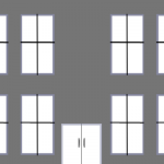
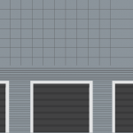
To begin, we’ll need images to use with our facade. For the purpose of the tutorial, we have two very rudimentary facades that were drawn in Photoshop. In your own facades, you can either do the same (drawing from scratch in an image editor), or you can use photos of real buildings–for instance, the buildings actually present at the airport you’re working on. Be sure that any photos you want to use are taken facing the building straight on. It will be difficult to set an image straight with any degree of realism if it was taken at an angle.
Note that your image files may be either PNG, BMP, or DDS format. The images do not have do be square. However, their dimensions in pixels must be a power of 2, as with all images used in X-Plane scenery.
Download the images for the tutorial here:
The image for our building facade
The image for our hangar facade
Understanding S-T coordinates
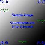
All image coordinates in X-Plane are specified in OpenGL’s S-T system. Within this system, every pixel in an image has a unique coordinate specified as a proportion of the width and height. This means that each dimension of the coordinate is between 0 and 1.
These coordinates are ordered as (s, t), which is (proportion of width, proportion of height).
The coordinate (0, 0) corresponds to the bottom left corner of the image, and the coordinate (1,1) corresponds to the upper right corner. Even if the image is not square, this is still true; the s coordinate is a proportion of whatever the width is, and the t coordinate is a proportion of whatever the height is.
Click on the images below for help in understanding this system:
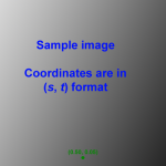
S and T coordinates illustrated
S and T coordinates illustrated in a rectangular image
Writing the facade file
The facade file itself is a text file containing information on the image and how it should be utilized in X-Plane. Let’s get started writing this file.
Create a new text document using your favorite text editor (e.g., Notepad, Emacs, Vi, etc.). Save it as FacadeNameHere.fac. In our example facades, we called them basichangar.fac and basicbuilding.fac.
Note: Except where noted, each line in the text file must be present exactly once–it may not be either omitted or repeated.
Specifying the file type
The first three lines of this text file should always be:
A
1000
FACADE
These lines tell X-Plane that it is indeed looking at a facade file.
Specifying which image(s) to use
Immediately following that is the line specifying the image resource to use. The image name should always have a path relative to the FacadeNameHere.fac file. For instance, in this example (taken from our example hangar facade), the image is in the same folder as the .fac file:
TEXTURE hangar.png
This is the recommended way to set up your folder, as it is the simplest way to do it.
If you have a so-called “lit” texture (a texture to be used at night, when the building would be lit artificially), you can use the following command immediately after the TEXTURE line:
TEXTURE_LIT ImageNameHere.png
The TEXTURE_LIT line may be omitted, as it is in our examples.
Setting the facade’s details
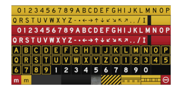
Following the TEXTURE command(s) is the RING line. If this is set to 1, the facade will form a closed loop, as is appropriate for buildings. When it is set to 0, it will be treated as an open loop, as is appropriate for fences.
Since both of our example facades are for buildings, we use the line:
RING 1
Next is the TWO_SIDED line. When this is set to 1, both the inside and the outside of the facade are drawn. This is appropriate if you have transparent areas in your image (for instance, in a window). When there is no alpha channel in your image, set this to 0, as is the case for both our example facades.
TWO_SIDED 0
Setting the level of detail
The level of detail command lets you specify how close to the facade the user must be for the object to be drawn. You specify both a lower and an upper limit. These distances are specified in meters. In both our example facades, we want the facade to be drawn unless the user is less than 0.1 meters away or farther than 50 kilometers away, so our files have:
LOD 0.1 50000.0
Everything following this line will be ignored unless the X-Plane user is in this range.
Note that you can use multiple levels of detail; in this case, you would have one LOD line, followed by all the other commands (ROOF, WALL, SCALE, ROOF_SLOPE, LEFT, CENTER, RIGHT, BOTTOM, MIDDLE, TOP), then another LOD line followed by the same set of commands. This would theoretically only be used to save memory. However, since facades only impact memory use in X-Plane, it would make much more sense to simplify one facade image and use it for all levels of detail–this is much more likely to save RAM than using two levels of detail.
Setting the roof texture
The ROOF command specifies coordinates in the image for use in the facade’s roof. The coordinates are an s and t pair (in that order).
The simplest roof texture is made up of a solid color. In this case, you need only specify a single ROOF command. The pixel found at that (s, t) location will be repeated across the whole roof. For instance, in our example facades, we use the pixel located at (0.1, 0.1) like this:
ROOF 0.1 0.1
If you don’t want a solid roof, you may instead use a whole portion of your image texture. In this case, you will have four instances of the ROOF command, each specifying one corner of the roof portion of the image.
For instance, if for some strange reason you wanted to use your whole image texture for the roof, you would do so like this:
Each wall line has a set of constraints defining when it can be used. The first number is the minimum width, the second number is the max width. These are in meters and define the range of walls in X-Plane that this wall definition can cover.
WALL 5 100
In this example, this facade will only be shown for walls that are at least 5 meters wide, and no more than 100 meters wide.
Scale & Slope
The scale of the texture in pixels is provided directly to X-Plane via a command in the file – it is not read from the actual texture file. This command defines the scale of the albedo texture used for walls – it is the number of meters the entire texture would fill horizontally, then vertically. For our hagar file we used
SCALE 40 10
X-Plane will use this reference to scale the image up or down since we specified in the line above that this texture can be used for walls between 5-100 meters wide.
The SLOPE command indicates the number of degrees the wall should bend.
ROOF_SLOPE 0
We set the roof slope to 0 to indicate there is no angle to it–our roof is flat.
Specifying the image’s “parts”
Now we need to specify what portions of the image will be used for each part of the facade. This will include a top, middle, and bottom, as well as a left, right, and center.
The bottom, top, left, and right divisions will be included once at most in each facade wall. Center and middle can be used repeatedly to provide particularly long or tall walls.
You will need to use your image editing program to determine the s and t coordinates of each of these lines. For instance, the ruler in Photoshop can be set to display in percent width and percent height, so you can easily determine the coordinates at which your image should be divided by WED.
LEFT 0.0 0.05
CENTER 0.05 0.365
CENTER 0.365 0.673
RIGHT 0.673 .958
BOTTOM 0.0 0.785
MIDDLE 0.785 0.977
TOP 0.977 1.0
Keep in mind:
Commands should be listed in order, e.g. all bottoms, then all middles, then all tops, then all lefts, then all centers, then all rights. (The left/center/right sequence may optionally come before the bottom/middle/top sequence, as it does in our examples.)
All coordinates must be adjacent, e.g. each “next” tile’s left or bottom coordinate must be the same as the previous tile’s right or top coordinate – no gaps! (The first CENTER line ends with 0.365 and the next CENTER line starts with 0.365.)
All facades should contain at least one horizontal and one vertical tile.
The completed text files
Basichangar.fac
A
800
FACADE
TEXTURE hangar.png
RING 1
TWO_SIDED 0
LOD 0.1 50000.0
  ROOF 0.1 0.1
  WALL 5 100
  SCALE 40 10
  ROOF_SLOPE 0
  LEFT 0.0 0.05
  CENTER 0.05 0.365
  CENTER 0.365 0.673
  RIGHT 0.673 .958
  BOTTOM 0.0 0.785
  MIDDLE 0.785 0.977
  TOP 0.977 1.0
Hangarwithroof.png
 A 800
 FACADE
 TEXTURE hangarwithroof.png
 RING 1
 TWO_SIDED 0
 LOD 0.1 50000.0
 ROOF 0.0 0.518
 ROOF 0.671 0.518
 ROOF 0.671 1.0
 ROOF 0.0 1.0
 WALL 15 200
   SCALE 30 15
   ROOF_SLOPE 0
   LEFT 0.0 0.049
   CENTER 0.049 0.364
   CENTER 0.364 0.671
   RIGHT 0.671 .975
   BOTTOM 0.0 0.393
   MIDDLE 0.393 0.440
   TOP 0.440 0.518
 WALL 0 15
   SCALE 30 15
   ROOF_SLOPE 0
   LEFT 0.671 0.7
   CENTER 0.7 0.8
   RIGHT 0.8 0.975
   BOTTOM 0.518 0.784
   MIDDLE 0.784 0.931
   TOP 0.931 1.0
Basicbuilding.fac
A
800
FACADE
TEXTURE buildingside.png
RING 1
TWO_SIDED 0
LOD 0.1 50000.0
  ROOF 0.1 0.1
  WALL 5 100
  SCALE 16 8
  ROOF_SLOPE 0
  LEFT 0.0 0.149
  CENTER 0.149 0.293
  CENTER 0.293 0.709
  CENTER 0.709 0.851
  RIGHT 0.851 1.0
  BOTTOM 0.0 0.426
  MIDDLE 0.426 0.915
  TOP 0.915 1.0
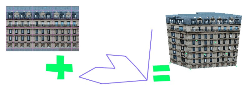
A facade is a special type of object in the X-Plane scenery system. Normally an object is specified as an OBJ file and placed in the scenery at a point and given a heading. With a facade, a facade specification text file (.fac) specifies what texture should be used for the object and how to build flat walls from part of the texture. The facade object is then placed in the scenery file along a polygonal path, and a building is extruded.
Facades allow you to specify a large number of buildings, each with a different shape, using one texture. The facade object is built from your facade specification text file in a smart manner, with the texture being replicated as well as stretched to look good at different sizes.
Facade concepts
A facade specification text file (spelled out in depth here) specifies how to build a facade object along a polygonal path. The facade text file specifies a texture; each facade object may (like OBJ files) use only one texture.
The DSF file will specify a polygonal path for the facade object and the number of floors to build; this lets each facade object be a different height.
A facade specification text file may designate a ring or chain facade. A ring facade object is a closed loop, which is useful for a building. A chain facade object is simply a set of connected links, which might be useful for a fence, etc.
A facade specification contains one or more levels of detail (LOD), or definitions for what the facade should look like at different distances. Each facade LOD specifies a minimum and maximum viewing distance. The various levels of detail must be continuous without gaps; the facade will not be drawn beyond the last level of detail. (This is the same as for OBJ files.)
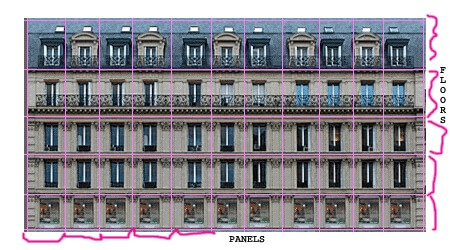
Each LOD for a facade specification is in turn made up of one or more walls. Each wall is broken into a number of horizontal divisions called panels, and vertical divisions called floors. Each wall specifies its panels and floors in terms of the texture for the facade object, as well as a resolution for the texture, to convert from pixels to meters. As a wall in the facade object is stretched or shrunk, panels and floors are added and removed to make the wall the right size. Each floor and panel in a wall can be specified as repeatable or non-repeatable, for visual control of the wall.
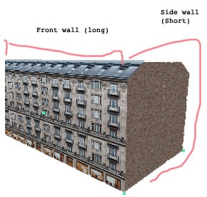
Each wall has a minimum and maximum length; as a facade object is built, x-Plane will look through every wall definition and randomly pick one wall whose length range matches the wall being built inside the sim. This allows you to specify one wall for short building sides and one wall for long building sides.
The roof of a facade (if specified) is always a solid color and is specified as a coordinate on the facade’s texture. Multiple roof coordinates can be provided, in which case X-Plane will pick one randomly.
The top floor of a facade can be sloped inward on a per-wall basis. Strange results may occur if the walls collide when angled.
How X-Plane Selects Facade Panels and Floors
The algorithm for selecting panels and floors is the same horizontally and vertically, and goes like this:
All end tiles are used before any middle tiles.
End tiles are equally balanced on both ends; for an odd number of tiles, the left/bottom end is preferred.
Only middle tiles can be repeated.
Middle tiles are used in left-to-right or bottom-to-top order.
Middle tiles will be split to match their left-right edges where possible.
Example: this horizontal stripe represents 9 panels: ABC = left panels, 123 = middle panels, XYZ = right panels. So the facade texture is organized as:
ABC123XYZ
This is the set of geometry created as the number of panels is increased; spaces represent X-Plane inserting an additional quad to form the shape.
A
A Z
AB Z
AB YZ
ABC YZ
ABC XYZ
ABC1 XYZ
ABC1 3XYZ
ABC123XYZ     <= exact match, only one quad
ABC12 23XYZ
ABC123 23XYZ
ABC123 123XYZ
ABC123 1 123XYZ
ABC123 12 123XYZ
ABC123 123 123XYZ
ABC123 123 1 123XYZ
Facade performance is typically limited by the amount of free memory, not framerate. That is, on most machines, a complex project with a large number of facades will exhaust memory before frame-rate becomes a problem. Most of these tips therefore focus on memory optimizations. (The smallest RAM footprint does also turn into lower vertex count, which is good for frame rate too.)
Correct Winding Order
Facades must be wound counter-clockwise, per the DSF specification. If your facade building’s roof is only visible when TWO_SIDED is set to 1, your facade is wound backward!
No Duplicate Vertices
Do not duplicate any vertices in the facade.
Do not repeat the first vertex as the last vertex; a square facade should have IS_RING 1 and contain only four vertices in the DSF. X-Plane will “close” your loop for you.
Avoid points in a facade that do not define the shape. For example:
1----2----3
|         |
5---------4
Point 2 should be eliminated for performance.
Sloped Roofs
Sloped roofs have some extra requirements:
No duplicate points, and no “straight” points (see above).
The roof is built out of a floor, so most times you will want at least two floors.
The roof should not fold in on itself.
If the facade is wound wrong, sloped roofs will not work.
Reducing Mesh Complexity
The facade engine can consolidate adjacent panels, but it must use more geometry to repeat panels. For this reason, it is best to make a facade wall that contains enough texture and panels to model the largest wall in your facade without repeating/duplicating texture space. A facade can be built in as few as 1-4 quads when geometry is cut, but if the panels are small, repeating the panels burns through a lot of memory.
The facade engine is most efficient when you do not use sloped roofs, the facade is convex in footprint, and the wall definitions match the real size of the facade both vertically and horizontally.
TWO_SIDED
Do not use TWO_SIDED for buildings; use one sided geometry and fix your winding order if necessary. TWO_SIDED is intended only for fences.
This tutorial will walk through the creation of an airport from scratch, including runways, taxiways, air traffic control frequencies, and more. It is related closely to the tutorial on airport customization; that document does not deal with modifying the airport data itself, and this one doesn’t deal with the terrain or objects placed on an airport.
Note that X-Plane’s official airport data is updated frequently, so you may want to check the Airport Scenery Gateway to see if there is an existing copy of the airport you’re building. For our tutorial, we’ll create data anew for Johnson County Executive Airport (KOJC), the same airport used in the Airport Customization tutorial.
This tutorial assumes you have installed the latest version of World Editor, selected an airport to work on, created a new scenery package, and familiarized yourself with the World Editor interface, all per the Airport Customization tutorial.
Remember to save often!
Getting Started
We begin with a new, empty scenery package. Before we can start laying down runways, we must first create a new airport. Open the airport menu and click Create Airport.
Click on the “unnamed entity” and give it a name–for our example, we’ll use “KOJC Johnson County Executive.”
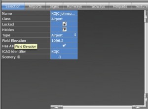
Now we need the airport’s elevation. (Note that, by default, this is in feet above mean sea level. You can change these measurements to meters by clicking the Meters option in the View menu.) Using the Airnav database, we can see that KOJC has an elevation of 1096 feet above mean sea level.
After inputting the elevation, uncheck the “Has ATC” box if necessary (by default, WED assumes the airport does have ATC). Then, type in the ICAO identifier–in our case, KOJC.
Entering the elevation for KOJC
Drawing the Main Runway
Now let’s draw the main runway. Using the Airnav database, we found that our example airport has its northern end at 38.8532228333 N, 94.7375677167 W, and its southern end at 38.8419830833 N, 94.737600583 W. We can use these coordinates, together with the mouse pointer coordinates at the bottom of the scenery editing pane, to zoom in on our airport.
Note that you may need to convert between degrees-minutes-seconds of arc to decimal degrees. In doing so, remember that there are 60 minutes of arc to a degree, and 60 seconds of arc to a minute, or use an online converter tool such as this one from the FCC.
Note also that you can place an orthophoto guide according to the Airport Customization tutorial to help visually check your scenery.
Now we will draw our runway. Select the Runway tool from the toolbar. Click once on one end of the runway, then again on the other end. For the sake of consistency, we recommend clicking first on the northern or western end (depending on the runway’s orientation) and clicking second on the southern or eastern end. Note that, for now, this does not have to be very precise–we’ll clean it up momentarily to make it pin-point accurate.
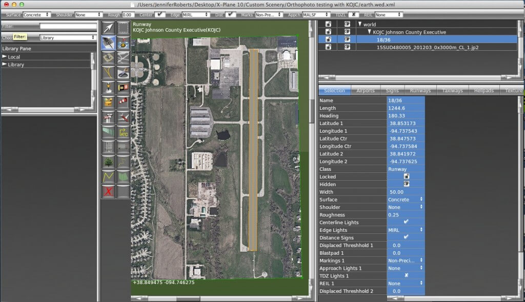
After your second mouse click, the green drawing line will turn into an orange outline, and the runway will appear in the object hierarchy pane, with a long list of attributes below it. Using data from Airnav (or another source if you prefer), you will need to input all the airport’s attributes. You should begin with the “Latitude 1” and “Longitude 1”–these are the coordinates of the first end you drew previously, which should have been the northern or western end of the runway. Then, input the “Latitude 2” and “Longitude 2” coordinates. (Note that the Latitude/Longitude Center, the Heading, and the Length attributes will all be calculated automatically from these.)
Beyond these attributes, the order in which you input the data does not matter. At the very least, you should specify the runway width, the surface, and, of course, the name.
Note that, for all attributes with “1” and “2” variants, the “1” end is the end you clicked first when drawing.
Some important attributes whose significance may not be obvious are:
Roughness: this specifies how rough the runway is (and how much it bumps the plane around) when taxiing. This is on a scale from 0.0 to 1.0. A runway in good condition should have a roughness of about 0.25.
Displaced Threshold 1 and 2: these specify how far from the end of the runway an aircraft is allowed to touch down, measured in feet or meters depending on your settings in the View menu. By default, the threshold is the end of the runway, so this is set to 0.0.
Shoulder: this sets the surface type of the runway shoulder, which is a small section of pavement beyond the runway found mostly in large airports.
Edge lights: runway edge lights are classified by the intensity of the light they produce. They can be HighIntensity Runway Lights (HIRL), Medium Intensity Runway Lights (MIRL), or Low Intensity Runway Lights (LIRL), or the runway may have no edge lights at all.
Markings 1 and 2: these specify the type of markings on each end of runway. Read more about these on Wikipedia.
Blast pad 1 and 2: these specify the length (in either meters or feet) of the blast pad. A blast pad is an area of pavement at the end of the runway constructed to keep dirt and grass from being blown around in the jet blast created by a large aircraft taking off.
Approach lights 1 and 2: many configurations exist for a runway’s Approach Lighting System (ALS). You can read about them here.
REIL 1 and 2: the Runway End Identifier Lights.
TDZ lights 1 and 2: the Touch Down Zone lights.
Our finished runway for KOJC looks like this:
The runway, with all attributes set
Repeat these steps for the creation of any other runways. You may want to lock the runways (by clicking the lock symbol next to them) in order to prevent accidental editing later.
Creating the Airport Boundary
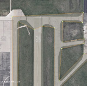
After creating your runways, select the Boundary tool (labeled with an image of a fence) from the toolbar. Click at each corner around the airport to draw the boundary. This is the area that will be flattened in X-Plane when the rendering options are set to do so.
Be sure to go in one direction–either all clockwise or all counter-clockwise. When you have placed the last corner, press the Enter key to commit the points to the boundary. At this point, the boundary will appear in the object hierarchy pane; you can then name it there.
If your points aren’t in the places you would like, you can use the vertex tool to click the points and drag them.
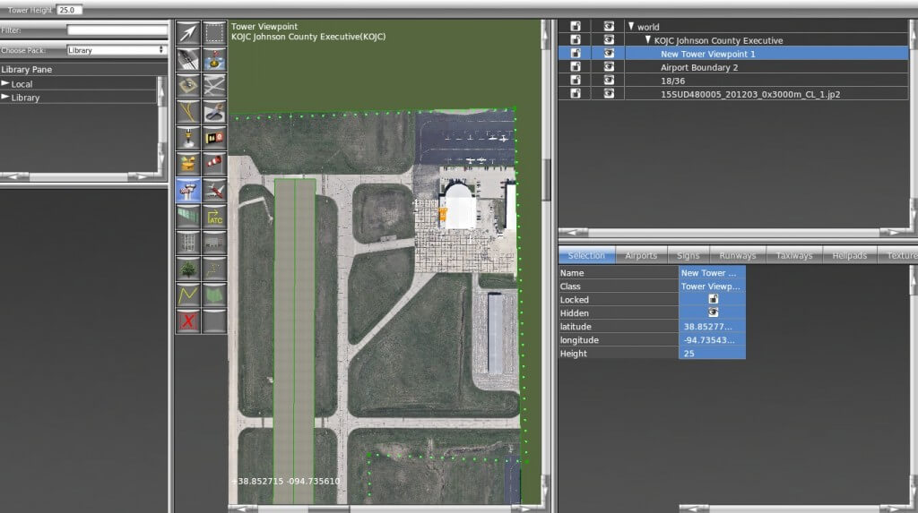
Setting the Tower Viewpoint
Select the Tower Viewpoint tool from the toolbar, and click where the air traffic control tower sits (as seen in the image below).
Setting the tower viewpoint
If there is no physical tower, as is the case in many smaller airports, set this to the main terminal. If this viewpoint is not set, selecting the tower view in X-Plane will put the view right on the runway.
After setting the viewpoint, be sure to set the Height attribute.
Creating Communication Frequencies
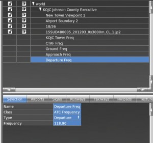
After creating your runways, highlight your airport in the Hierarchy pane by clicking on it. Open the Airport menu and click Create ATC Frequency.
An “unnamed entity” will appear in the object hierarchy pane. Name this one something like “[Airport] Tower Freq,” and set its attributes properly (once again, this information can be found in the Airnav database). For instance, we found that KOJC’s tower uses frequency 126.0, so we set its attributes accordingly.
Repeat this for all the communication frequencies present in your airport, using the Type attribute to specify which frequency it is. In our example airport, we have 5 different radio frequencies to set up, using the Type attributes CTAF, Tower, Ground, Approach, and Departure. In the following image, we have set the KOJC Departure Freq to Departure type and are setting its frequency at 118.9.
Setting the Departure frequency
It may be helpful for the sake of organization to group these communication frequencies together. To do so, highlight the frequencies you want by clicking them while holding down the Ctrl key in Windows or Command key in OS X. With them all selected, go to the Edit menu and click Group.
Name this new group, and we’re ready to move on.
Drawing Taxiways and Other Pavement
Now let’s draw your taxiway(s) and other pavement (aprons, parking lots, etc.). We will use the Taxiway tool to do all this–X-Plane doesn’t care that a layer of asphalt might actually be a parking lot.
Note: when drawing these polygons, make sure there is only one enclosed area per polygon–that is, make sure that the outline does not cross over itself at any point.
With this in mind, select the Taxiway tool from the toolbar and click around the outside of your paved areas. At this point, you should not be making the shapes look pretty–use a small number of nodes, with the intention of cleaning the shape up later. Note especially that you do not need to pay special attention to curves–soon we will create bezier curves to follow the contours of the pavement, but don’t worry about it now.
The best way to do this is to outline all the taxiways and other pavement in your object, then use the Hole tool to cut out all the area that gets selected which isn’t pavement. When you finish drawing each item, press enter–you should have a few objects that look similar to those in the image below. This will not work if you need markings on your (true) taxiways, though–in that case, you’ll need separate objects.
If you are using an orthophoto, it will be helpful to change the transparency of the taxiway in order to see where the holes should be drawn. To do this, click the View menu and select “Pavement Transparency.” Set the taxiways to 50% transparency for a good balance.
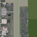
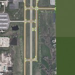
In the image on the left below, the taxiway has just been drawn–it covers a lot of area that it shouldn’t. Then, in the image on the right, holes have been cut in it so that it doesn’t cover the grassy areas around it. It still isn’t pretty, but we’ll clean it up soon to more closely match the real taxiways.
A newly drawn taxiway covering areas it shouldn’t
A taxiway with properly drawn holes
Smoothing the Curves
Now that we have (very) basic outline of our pavement drawn, we need to modify it to follow the contours of the actual airport’s curves. We’ll do this by turning the node near a corner into a bezier node, which will cause the line connected to it to curve around it.
You may need place an extra node between two points for the purpose of creating this bezier node. To split the line connecting two points and place a node between them, highlight the points using the vertex tool, open the Edit menu, and click Split. Alternatively, you can highlight the points and press Ctrl+E in Windows, or Command+E on a Mac.
For instance, in the image below, we split the line between the node on the left and right, then used the vertex tool to drag the new node down to the pavement.
A new node created by splitting
Now, to turn this into a bezier node, hold down the Alt key and drag the mouse away from the point. After you let go of both the mouse and the Alt key, you can click and drag the outside arrows to further tune the curve.
Alt-click and drag the nodes
From here, you can click and drag the arrows attached to the node to further modify the curve. A completed curve will look like the above image.
Repeat this process for each curve around the pavement.
Creating Markings and Lighting
Now we will add markings to our runways, taxiways, and other pavement. Markings come in two varieties–perimeter markings (found around the outline of taxiways), and overlay markings (like taxilines, ILS, and hold short markings).
Note that whenever you select a tool that supports markings (i.e. the taxiway and taxiline tools), you’ll notice some options appear at the top of the scenery editing pane. One of these options are markings. When you select a marking in this pull-down menu, that marking will be applied to that tool until you change it. So if you were going to draw taxilines, you’d select the taxiline tool, then set the Markings to Double Solid Yellow (Black) and begin drawing the shape.
You can, however, draw the shape first and add the markings later. This is easily accomplished by selecting the entity, with either the vertex tool or the marquee tool, then going to the attributes pane and setting the Line Attributes, Light Attributes, or both. When you do this, the markings will be applied to the entire shape. This is generally not what is desired, though, and you’ll need to remove the markings from some of the segments for taxiway intersections and the like.
To remove the markings from one section of the taxiway, select a single node using the vertex tool. Then, in the attributes pane, set its Line Attributes to none. The line connecting this node to whichever node was drawn after it will no longer have that attribute. For instance, if you selected Node 9 and set its Line Attributes to none, the line connecting it to Node 10 would have no markings.
Adding the Finishing Touches
We have just a few more things to add to the airport for it to be ready to go.
Creating Runway Signs
To create a runway sign, select the Sign tool from the toolbar. Click where you would like to place it, then drag your mouse around that point to orient it in the direction it needs to go. Note that the arrow coming out of the sign indicates its heading. To move a runway sign, use the marquee tool to click and drag it. To change its heading, drag it with the vertex tool.
For information on setting the text on the sign, and for examples of the text used, see the WED manual appendix on defining taxi signs.
Creating Windsocks, Light Fixtures, and Airport Beacons
Windsocks, light fixtures, and airport beacons are all placed on the airport like runway signs–click to place them, and, in the case of the light fixtures, drag the cursor to change their orientation. You can use the marquee tool to change their position, and, for the light fixtures, you can use the vertex tool to change their heading.
Adding ATC Flow and Taxi Networks
If you are customizing a large or busy airport, it is a good idea to specify the taxi network the airport should have, as well as the ATC flows. A taxi network you create is more likely to be realistic than the one X-Plane can automatically generate. Most large airports will also have several “flows” depending on weather or time conditions, or type of aircraft
To add an ATC flow item, select your airport in the hierarchy pane, open the Airport menu, and click Create Airport Flow. Then, after selecting that flow in the hierarchy pane, open the Airport menu again and select Create Runway Use Rule, Create Runway Time Rule, or Create Runway Wind Rule.
These rules specify under what conditions the runway should be used. X‑Plane will try to use the rules in order (from top to bottom), so be sure to order multiple flows from most specific to least. It also a good idea to have a generic, catch-all flow that can be used in all conditions in case the condition-specific flows overlook a possible scenario.
To create taxiway routings for the AI aircraft, select the taxi routes tool. Set your properties at the top of the window, then click to trace the path aircraft should take. The Departure, Arrival and ILS fields set up hold short parameters. The slop field indicates how close your point must be to another taxiway section in order to snap to it. Larger numbers allow the paths to snap together from farther away. The other preset fields are self-explanatory.
Check for degenerate edges, double nodes, and crossing edges before exporting an airport with a taxi network. These are found under the Select menu and will show any errors in the attributes pane.
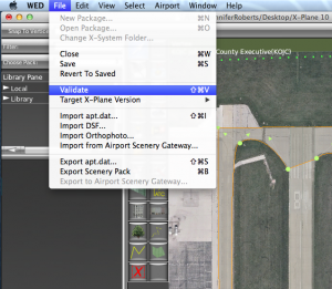
Before exporting your airport data, open the File menu and click Validate, as shown in the image below.This command will check the WED file for errors based on the current export target. You can change the export target by selecting Target X‑Plane Version from under the File menu. Remember that selecting a version older than 10.0 might disable newer features, such as ATC data.
File –> Validate
If no errors are present, select Export Scenery Pack from the File menu. The new scenery will be visible the next time you load the area in X‑Plane.
Alternatively, with version 1.3 of WED and newer, you can upload your scenery creation directly to the Airport Scenery Gateway. See these instructions to register first.
This tutorial will walk through very basic customization of an airport’s scenery using freely available tools. It is targeted at first-time users of the scenery tools–no prior experience is required or assumed. Screenshots were taken in Windows 7 or OS X Mavericks, but the steps should be identical in other versions of Windows or OS X, except where noted.
The tool that we will be using primarily is WorldEditor (or WED), which was created by Laminar Research specifically for working with X-Plane scenery. If you do not already have the latest version installed on your computer, you can download it here.
Once the file has downloaded, unzip it to an easy-to-find folder. No installation is required; to launch it, just double click WED.exe (Windows) or WED.app (OS X). Because there is no installation, we recommend placing the file in the X-Plane folder to make it easier to find.
Special considerations for Windows Vista/7 users
In Windows Vista and Windows 7, users may need to disable Aero for their mouse clicks to be where they appear to be. In some cases, unless Windows is forced to use the Basic theme, clicking in the WED window may act strangely.
To launch WED using the Basic theme, right click on WED.exe and click Properties from the menu that appears. In that window, go to the Compatibility tab and check the Disable desktop composition box (highlighted in the image below). Click Apply, and in the future, WED will always launch using the Basic theme.
The Compatibility tab for the WED executable
Select an airport
Before we can begin, we’ll need to select an airport. Regardless of what airport you are interested in customizing, be sure to search the web (and especially the X-Plane.org Downloads page or the Airport Scenery Gateway) to make sure someone else hasn’t already created a good scenery package. There’s nothing worse than spending hours on a project, only to find that there is a better free version of it already available!
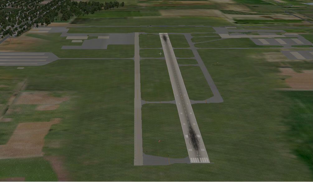
For the purposes of this tutorial, we will work with Johnson County Executive Airport (KOJC) in Kansas. As you can see in the image below, the default X-Plane scenery is detailed regarding the placement of runways, but is unimpressive beyond that–a perfect candidate for basic customization!
KOJC as it looks by default
Creating a new scenery package
We are now ready to create a new, empty scenery package in WED. Double-click on WED.exe (or WED.app on a Mac) to launch it.
When the WED window appears, you may first need to navigate to your X-Plane folder, but then you should be able to click the New Scenery Package button. Type a name for the package, then press Enter. For our example airport of Johnson County Executive, we’re going to use the name “KOJC Johnson County Executive.”
With the name entered, click Open Scenery Package. After a moment, the WED drafting window will appear.
Getting familiar with the workspace
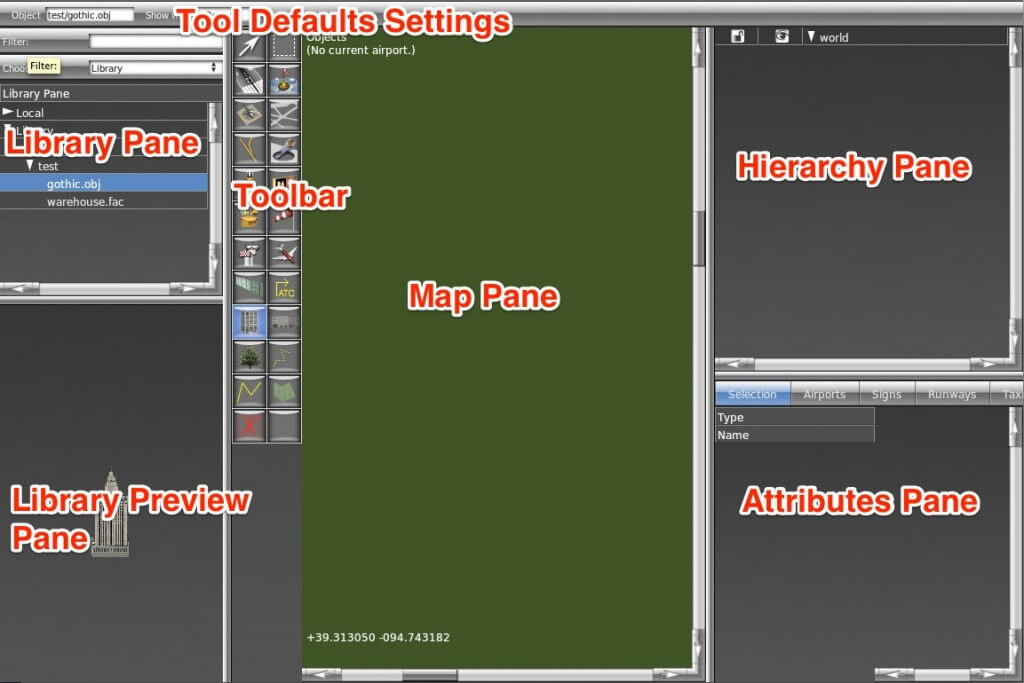
The WED workspace is made up of multiple panes, labeled in the image below.
On the far left is the library browser. Here, you can browse through the files in the X-Plane library using their virtual paths. (A full understanding of the library system is not required for our purposes here, but for further reading, see The X-Plane Library System). We will talk more about this pane when we begin adding objects to our airport.
To the right of the library browser are the scenery editing panes This includes the toolbar in the left of the pane, the pointer coordinates at the bottom, and the map pane in the center. This pane is used to place objects and to visually modify their positions. To zoom in, either scroll up with your mouse or press the + key on your keyboard. To zoom out, scroll down or press the – key. Note that the program will zoom in toward wherever the mouse is pointing.
To the right of the scenery editing pane is the object hierarchy list and the attributes pane. The object hierarchy pane lists all the objects in a given airport, in (roughly) the order that they will be loaded in. In reality, X-Plane will load certain sets of objects together (for instance, all of the taxiways), but for most purposes, the order of objects in this pane is the order in which they will be visible in the sim. The objects at the bottom of the list will be covered by all the things above them, and objects at the top of the list will be visible above all the objects below them.
Note that in this pane, each object and each group of objects can be set to locked (and un-editable) or unlocked (and editable), and visible or invisible by clicking the appropriate icon. In the image above, all objects are unlocked and visible.
Beneath the hierarchy pane is the attributes pane. This lists all the user-modifiable attributes of whichever object is selected. Click the field to modify its value.
Above all these panes is the tool defaults pane, where you can set up the preferences before using a tool so you won’t have to edit later. The attributes available to set vary by tool but will be remembered the next time you use it.
When the WED window opens for the first time, the size of the window’s panes may not be to your liking. To fix this, mouse over the bars separating each segment and drag it to the size you would like. Alternatively, you can right click within the three outer panes and drag your cursor to resize that pane (doing this in the center pane will just move the view).
Importing airport data
With our package created, we’ll need to import its apt.dat information. Recall that an apt.dat file contains information about the layout of an airport. The airport data included with X‑Plane by default is generally of high quality, even in cases such as this where only the main runways are included, so we will import the existing data for KOJC.
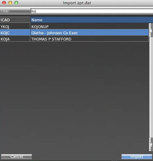
Open the File menu and click Import from Airport Scenery Gateway. We recommend using this option because it contains the most up-to-date airport information.
Type the ICAO identifier KOJC in the text box labeled Filter (found at the top of the dialog box), click the airport to select it, and click Next. Select the specific scenery pack you want to edit on the next screen, then click Import Pack(s). (In cases where more than one scenery exists at an airport, select the pack with the status “Recommended.”)
Selecting KOJC for import
You should now be able to see, at the minimum, the main runway and an airport boundary.
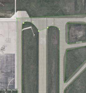
Adding an orthophoto guide
Depending on the airport you’ve chosen, you may not be familiar with how all of its buildings, pavement, and so on are laid out. We can fix this by downloading some orthophotos of the area–aerial photos whose corners are mapped to exact latitude and longitude coordinates.
For scenery in the US, it’s easy to obtain public domain orthophotos that may be used freely in our scenery. Outside the US, it may be more difficult–copyright on most imagery like this will prevent you from distributing the images with your scenery.
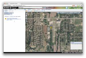
Since our example airport is in the US, we’re going to download our orthophoto from a public image server, the USGS Seamless server. For instructions on how to download the images you need from this server, see the Using the USGS Seamless Server article.
From here on, we will assume that you have either downloaded orthophotos from the Seamless server, or that you have similar files from some other resource. The advantage to using the Seamless server is that many of the image file types have their geographic coordinates embedded in the files themselves–they are GeoTIFFs or JPEG2000s.
KOJC on the USGS Seamless Server
Once you have your orthophotos saved into your custom scenery folder, click Pick Overlay Image… from under the View menu, and navigate to your image file. Assuming you selected an image with coordinates embedded in the file, WorldEditor will automatically place the image in the correct location. Now as we complete the next steps of adding objects and facades, we can use the orthophoto guide to help us place them in the correct spots.
Note: The overlay image is only a guide for use in WorldEditor and will not show up as orthophoto scenery in X-Plane.
Adding objects
With our basic data imported, it’s time to build up the airport’s objects.
For the purpose of this tutorial, we don’t want to design our objects from scratch. Instead, we will use X-Plane’s built-in objects. We will not be using the OpenSceneryX object package, as it would prevent us from uploading our finished scenery to the Airport Scenery Gateway database.
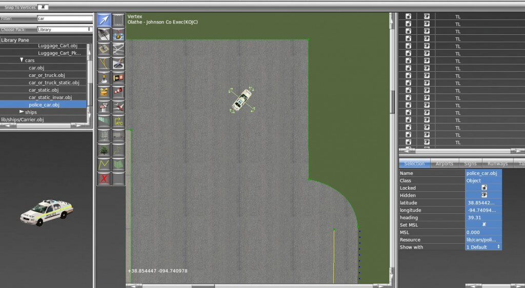
Let’s begin adding our objects. To draw an object, first find it in the library pane. Use the library drop down menu and the “Filter” field to narrow down the scope of the search (for example, by typing “tower” if you are looking for a control tower). Select an object by clicking on it in the list, which will also select the Object tool from the toolbar. You can use the mouse to drag your view around in the preview pane if you are not familiar with what the object will look like in X-Plane.
Click in the map pane to place it, or click and drag your mouse around to set the object’s heading at the same time. You can also use the vertex tool to change the heading, and use the marquee tool to drag it around (click on the cross). If you’d like, you can change the name of the object by clicking twice on it in the hierarchy pane or in the name field of the attributes pane.
Rotate an object using the vertex tool
Drawing facades
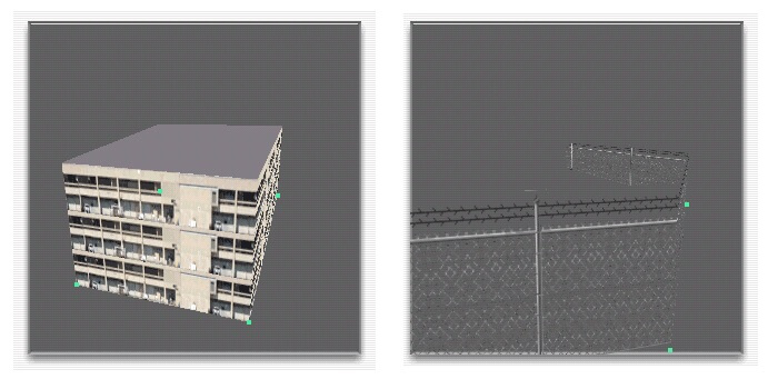
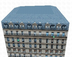
A facade in WED is essentially an image wrapped around a polygon at a specified height. This is used to build a simple building quickly and easily. Users specify only the shape of the building at its base, its height, and the .fac file to use.
To draw a building facade, select the facade tool from the toolbar or select a .fac file from the library pane, which will automatically select the correct tool.
Use the facade tool to trace the outline of the buildings you’d like to add. After it is outlined, give the facade a name and change its height (in the attribute pane) as needed.
Exporting a scenery package
When you have finished customizing the airport, open the File menu and select Validate. This command will check the WED file for errors based on the current export target. You can change the export target by selecting Target X‑Plane Version from under the File menu. Remember that selecting a version older than 10.0 might disable newer features, such as ATC data.
If no errors are present, select Export Scenery Pack from the File menu. The new scenery will be visible the next time you load the area in X‑Plane. If you would like to share your work with other X-Plane users, check out the section of the manual that details how to submit scenery to the Airport Scenery Gateway.
> 💡 NOTE: X-Plane’s Taxi-Sign Specification was originally a joint effort between FlightGear and X-Plane and applicable to both simulators; however, X-Plane has evolved in a differing direction and this specification may no longer be applicable to Flight Gear.
General
3D Taxi-Signs in X-Plane are auto-generated, and the glyphs (letters and symbols) on each Taxi-Sign are rendered from a text string of ASCII characters called a taxi sign stringorsign string. S_ign strings_ for each Taxi-sign are part of the apt.dat file.
Sign strings are case sensitive! When we write “A-Z”, we mean upper case letters. When we write “a-z”, we mean lower case letters.
Sign strings may contain NO new line characters and NO whitespace characters (tab, spaces)
Example Taxi Sign String: {@L}P2{@R}16-34CAT{r1}{@Y}{@@}{^lu}P2{@L}P2
Glyphs
A glyph is simply a graphic shape that means something. The letters of an alphabet are glyphs. Symbols are glyphs. Egyptian hieroglyphics are glyphs, etc. We use the term glyphs here because a Taxi-Sign contains more than just letters in an alphabet. The image below shows all the possible Taxi-sign glyphs that are available in X-Plane.
A Taxi-Sign glyph is represented / encoded by either a single ASCII character (single-char-glyph) or a ASCII character sequence (multi-char-glyph). We call these encodings glyph-strings; therefore, a Taxi-sign’s contents are rendered from a taxi sign string, which further consists of individual glyph-strings.
Curly Bracket Pairs
Curly brackets are used to bracket either Control Directives, or multi-char-glyphs. The following rules apply to the use of curly braces
Every open curly brace must have a closing curly brace.
Curly brace pairs must not be empty.
Nested curly braces are not supported.
Control Directives:
Control directives are two-character sequences in brackets that tell X-Plane which color category of Glyph to use, as well as delimit what is on the front and back of the sign. Control directives for the color category are modal, meaning all glyphs after that directive will use that color until another color directive is specified. There are five directives available as follows:
Directive
Description
Glyphs Supported
@Y
Use Yellow background set
Supports all valid glyphs
@R
Use Red background set
Supports all valid glyphs
@L
Use Black background with yellow chars
Supports only A-Z, 0-9
@B
Use Black background with white numbers
Supports only 0-9
@@
following glyph strings for back of sign
Single Char Glyphs
Single char glyphs are represented by a single ASCII character, for example A, –, 6, etc. The following are valid single letter glyphs:
Character
Description
A-Z
Capital Letters A thru Z
0-9
Integers 0 thru 9
-
produces a hyphen
*
produces a dot
.
produces a period
,
produces a comma (when used outside brackets
/
produces a slash separator
_
produces a space
Multi Char Glyphs
Multi char glyphs are glyphs that are encoded using more than one ASCII character. Multi char glyphs must be contained inside curly brackets unless the Taxi Sign String qualifies for Comma Delimited Syntax. The image below highlights the glyphs that use multi char glyph strings.
The following table lists the multi-char glyph strings:
Glyph String
Description
^u
Up Arrow
^d
Down Arrow
^l
Left Arrow
^r
Right Arrow
^lu
Left Up Arrow
^ru
Right Up Arrow
^ld
Left Down Arrow
^rd
Right Down Arrow
r1
Roman Numeral I
r2
Roman Numeral II
r3
Roman Numeral III
no-entry
“Do not enter” symbol
critical
ILS Critical Area Boundary sign
safety
Runway Safety Area
hazard
Taxiway Ending Marker
comma
For an actual comma on the sign
> 💡 NOTE: The character, ^ is only valid when used with the multi-char glyph strings above.
Fixed Glyphs
Fixed Glyphs are those glyphs that always appear the same, regardless of the active color directive. The following are the fixed color glyphs: hazard, safety, critical, no-entry
Divider Line
The Divider Line is a special glyph, encoded by the pipe symbol, ‘|’, and having some special rules for its use. Below is an example of two signs, one with and one without the Divider line. The Taxi Sign String used to produce each sign contents is also given.
{@Y}BOOK|CASE{@Y}BOOKCASE
The following conditions apply to use the Divider Line / pipe symbol
A Divider Line must have the same color glyphs on either side of it.
e.g. {@Y}BOOK|{@R}CASE is illegal.
The Divider Line only works for @Y, @R, and @L color modes. Any pipe symbol following a @B directive is ignored.
A divider line cannot be:
next to a Fixed Glyph
next to another Separator Line
at the beginning or end of a sign side.
Comma Delimited Syntax
When a Taxi Sign String only contains a single directive, then the Taxi Sign String may be fully contained within a single set of curly brackets along with the one Control Directive; however, each glyph string after the directive must be comma delimited. This reduces the amount of curly brackets required for single sided signs with only one color mode, e.g.
{@Y,^lu,TERMINAL,|,CARGO,^ru}
Unsupported Characters
!
“
#
$
%
&
‘
(
)
[
]
+
:
;
<
=
>
?
~
b
g
j
k
q
v
w
x
Example Taxi Sign Strings
{@L}A
{@Y}{^l}C
{@Y}17-35{^r} or {@Y,17-35, ^r}
{@B}1 or {@B,1}
{@R}11-29 or {@R,11-29}
{@L}B7{@R}10CAT{r2}/{r3}
{@Y}{^lu}B{@L}C{@Y}C{^u}|F{^r}
{@Y}WEST_APRON{^r} or {@Y,WEST_APRON,^r}
{@L}P2{@R}16-34CAT{r1}{@Y}``{@@}{^lu}P2{@L}P2 (Front Side – blue text)
{@L}P2{@R}16-34CAT{r1}{@Y}{@@}``{^lu}P2{@L}P2 (Rear Side – blue text)
> 💡 The following table is a table of Control Directives that are only used for error reporting and internal usage. They cannot be used by hand.
@I
Glyph specific
These are the Fixed Glyph Signs: critical, no-entry,safety, and hazard and cannot be declared by hand
@P
Represents a pipebar, only for error reporting
Indicates the glyph is a pipe bar and should be checked if valid
@X
Only for error reporting
Indicates that parsing stopped before any valid color has been found