Beginning with X-Plane 12.3+, there is a new Weather (WX) radardisplay with advanced behaviors available to aircraft authors. The old, legacy composite WX display is still available as well. The new display is available in two forms. For aircraft authors, the first form is displayed via the regular EFIS map instruments found in PlaneMaker's instrument library. For plugin authors, the second form is via a 2D RGBA return-strength texture, which provides radar return strength values in the 8-bit RED channel of the texture, from which plugin authors can read these values and render their own wx displays. Other channels in the return-strength texture are not currently used.
The radar display on X-Plane’s EFIS maps is rendered to a 24bit RGB image using a generic color stripe texture.(Resources\bitmaps\world\maps\RADAR.png). No particular effort is made to make the radar look like any specific make and model, but rather is made generically plausible to NEXRAD / FAA standards. You can customize this texture for your specific aircraft if you like by duplicating the stripe texture into a EFIS subfolder in your aircraft’s cockpit folder (not cockpit_3d) and modifying it.
About Aircraft Radar
Aircraft radar systems typically consist of a single antenna, a Processing CPU, a graphical display and various mode controls. The antenna scans a Sector Arc within the antenna’s Sweep Arc at a rate called the Scan Rate, and receives return signals which are processed and shown on a WX Display in the cockpit. The WX display screens are updated at a rate called the Refresh Rate, which most of the time, is the same as the Scan Rate, but not always. (more below)
The Sweep Arc is the maximum arc range the antenna can physically traverse, whereas the Sector Arc is the arc range actively being scanned. Most of the time, the Sector Arc = Sweep Arc for generic scanning; however, some systems have the ability to narrow the Sector Arc, in order to achieve a higher scan rate in a particular direction. The video below shows an antenna moving through its Sweep Arc.
<future image of radar_sweep in new docs>
Many radar systems have antenna that can tilt up/down over a small range of angles. In simple systems, this tilt angle is manually controlled by the pilot (Manual-Tilt). In slightly more sophisticated systems, the tilt-angle can also be adjusted up or down automatically based on other factors such as pitch attitude, altitude, range settings, etc. (Auto-Tilt). In even more sophisticated systems, the antenna can automatically scan at multiple tilt angles and use those multiple scans to generate a single composite image to display to the pilots (Buffering Types). The video below shows an antenna scanning through multiple tilt angles in such a mode.
<future image of multi-scan opt in new docs>
GA aircraft usually have one WX display whereas Transport Category Aircraft requiring two pilots commonly have two WX displays, one for each pilot. When two WX displays exist, one for each pilot, then each display may have its own set of controls, and when the tilt angles for each side differ, then the radar antenna is “time shared” between the displays and the Refresh Rate on each WX display then becomes <u>half</u> of the antenna Scan Rate. X-Plane can simulate Manual-Tilt, Auto-Tilt, Multi-Scanning and time shared antenna behaviors, as well as many other modes.
PlaneMaker Settings
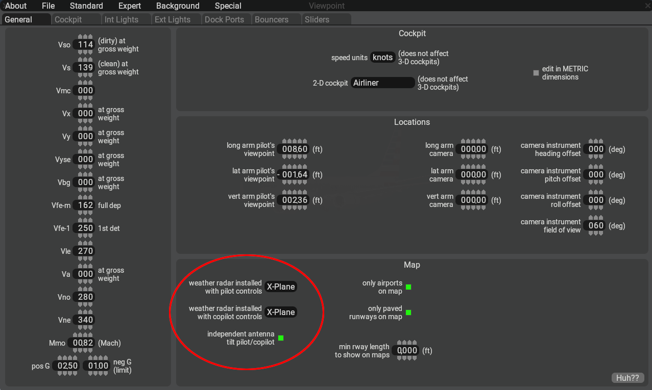
To implement the new radar, you will need PlaneMaker 12.3.+ There are three configuration settings, located in the Standard Menu > Viewpoint > General Tab > Map Panel as shown below.
Each of the two pulldown menus contain the following three options:
Option
Description
None
Legacy radar image used on EFIS map instruments.
X-Plane
New radar image used on EFIS maps instruments. (using new controls/DRs/commands)
Plugin
Radar emission “return strength” values are provided via a 8-bit grayscale texture for plugins to query. (The grayscale texture may be viewed on the PM EFIS instruments.)
When both the pilot and copilot pulldowns are set to ‘X-Plane’, then a checkbox for independent antenna tilt will become available, otherwise it will be hidden. As mentioned above, when this option is enabled and the pilot/copilottilt control settings differ, then the single antenna will be time shared between the radar controls. When this option is not checked, then both WX displays will use the same tilt value. Any input on either side will be copied to the opposite side.
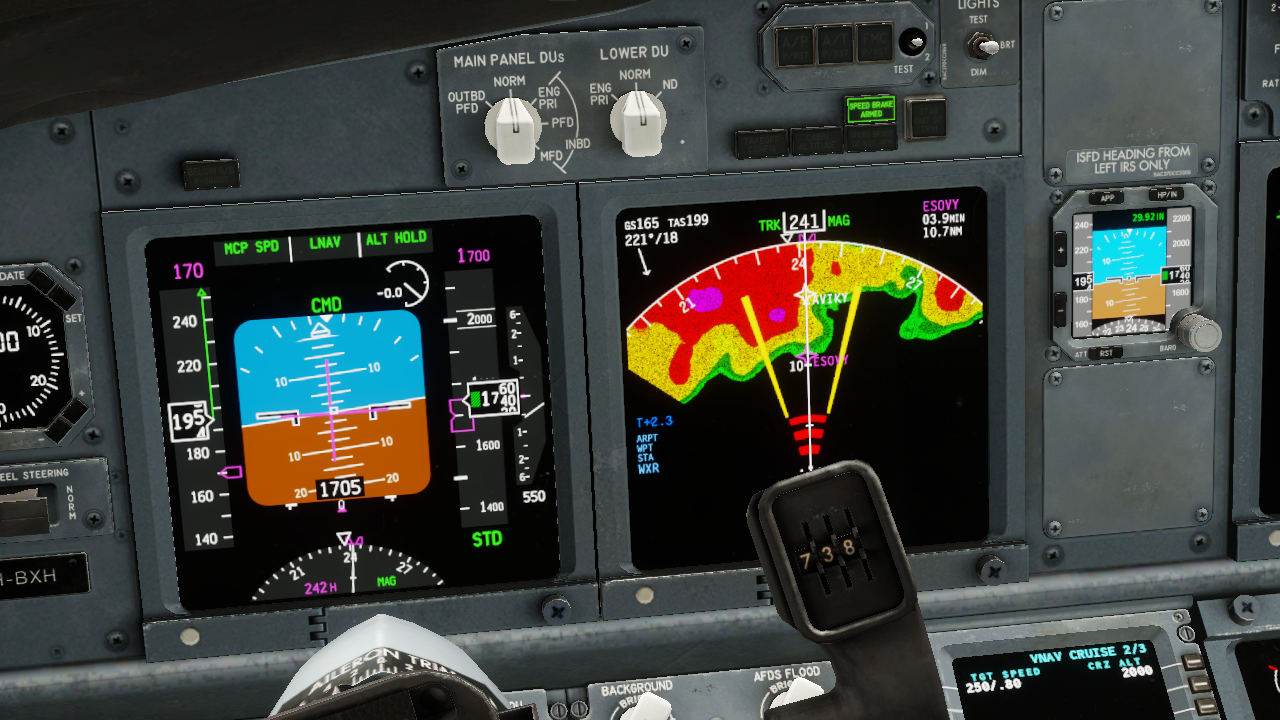
The WX radar image is rendered on PlaneMaker's EFIS map instruments as shown below. These instruments can depict either weather or EGPWS terrain depending upon the EFIS control settings. WXR and EGPWS TERR modes (described further below) are mutually exclusive and cannot be displayed at the same time.
> NOTE: If you need EGPWS functionality, then this requires a GPS FMS instrument to be present on the 2D or 3D panel for X-Plane to load the terrain database. If your panel texture space is limited, you can use one of the screen only GPS FMS instrument options and scale it down via its Size parameter so it takes up very little texture space.
> If only WX Data is desired, with no map overlays, such as would be the case for an older, dedicated WX Display unit like a Collins IND-300 or Bendix RDS-81, then you should use the basemap_s_HM.png instrument. This instrument only displays Weather or Terrain data exclusively and is suitable for overlaying other generic or plugin generated graphics.
Plug-In Customizations
For those desiring to craft their own WX display graphics and having selected the PlugIn pulldown option in PlaneMaker, the virtual radar return strength values are written into the 8-bit RED channel of a 32-bit RGBA texture (GBA channels not used). The 8-bit value at every point represents the strength of the radar return on a scale of 0 to 255. A plugin can use this texture data to further generate and render a color grading exactly representing a particular model of radar.
The plugin can either draw to the panel texture (legacy method), or draw to an FBO of a custom avionics device using the XPLMAvionics API, which is the preferred method for plugin EFIS graphics since X-Plane 12.1. Via the XPLM Avionics draw callback, a plugin can call the XPLMGetTexture() function with the enum values xplm_Tex_Radar_Pilot or xplm_Tex_Radar_Copilot to access the texture values for subsequent graphics customization.
Operating Mode Descriptions
Before getting into the Datarefs and Commands sections below, it is helpful to discuss the various Operating Modes that Radars can employ. The table below lists all the modes available to simulate Radars of varying complexity. The modes you implement will depend upon the model of Radar you are simulating.
The Datarefs and Commands to implement the various modes are listed further below, as are additional descriptions of the various Radar types and their features.
> Note that enabling the radar on the ND (sim/cockpit2/EFIS/EFIS_weather_on) will not turn on the radar. The ND will remain empty until a discrete radar mode other than OFF is selected. > > When a new flight is started with engines running, the radar will default to WX+T mode, with stabilization, predictive windshear, and auto-tilt functions turned on.
Mode
Description
OFF
In this mode, the radar is not powered, the antenna does not move, and the radar image texture is cleared to all black. This is the default setting for cold & dark starts
TEST
The radar is powered in standby but not emitting radiation. A test image is displayed on the screen showing the color band of the radar.
WX
The radar is emitting radiation and sweeping the antenna left and right at the selected tilt. It detects liquid water in the air, once the droplets have reached a sufficient size. This is why it sees cumuliform clouds, which consist of comparatively large droplets, but it can't detect stratiform clouds that are dominated by very small droplets. Only when the drops become large enough to fall out as precipitation will the radar pick up stratiform clouds. The radar cannot detect small, dry ice crystals. The tops of cumuliform clouds can reach up into very cold temperatures in the atmosphere, where the upper part of the cloud will consist of ice crystals instead of liquid water. This is called glaciation. The radar's ability to detect these very cold particles is very limited. They can only be seen at very high gain settings, if at all. That is why the gain is increased with altitude (decreasing temperature) when left in the auto (calibrated) position. Because of the low reflectivity of dry ice crystals in very cold air, it is possible to "overscan" cumulonimbus clouds when the radar scans only the upper portions of them, where it doesn't get a return. It is therefore necessary to tilt the radar down to scan the lower, warmer portions of cumulonimbus clouds where liquid water generates a strong return. Auto-tilt in cruise flight takes care of that by tilting the radar down. A good technique to detect cumuliform clouds from higher altitudes is to tilt the radar down until you can see the ground return at the edge of the display. Cumuliform clouds are then easily detected as they "walk out" of the ground returns. Ground returns appear when the radar beam touches the ground. Note that the beam is about 3degrees wide in either direction, so the edge of the beam touches the ground about three degrees below the actual tilt setting. The angle at which the beam strikes the ground determines the strength of the return, not the height of the elevation. Flat ground creates only weak returns, while steep mountainous terrain creates very strong returns. Ground returns will appear unless you are using ground clutter suppression, as explained below.
WX/T
The same as WX, but the areas of most severe turbulence are colored magenta. Note that turbulence detection still needs humidity. Clear-air turbulence such as orographic turbulence or jet stream shear are not detected.
TURB
Only shows magenta areas of most severe turbulence
MAP
In ground mapping mode, the radar beam is spread vertically, to scan a broader range of ground in front of the aircraft. The gain is adjusted down so less weather is picked up. Again, the strength of the ground return reflects the steepness and ruggedness of the terrain, not the elevation. MAP mode turns off any multi-scanning altitude mode, as it is normally used for ground mapping, not for examining weather at high altitudes. Selecting MAP mode turns off ground clutter suppression, if it was previously selected.
MULTI-SCAN – Auto
For Multi-Scan Buffering Radars (see Buffering Types below). This mode corresponds to flipping the multiscan switch to auto on a Rockwell/Collins multiscan radar. The tilt will be automatically controlled and scan a high and low tilt in front of the aircraft, to capture weather in a wide range of altitudes. The tilt angle displayed corresponds to the average tilt used. When OFF, the ‘nominal’ tilt-angle may be manually controlled.
ON PATH
For Elevation Buffering Radars (see Buffering Types below). This mode corresponds to setting the mode selector to AUTO or ON PATH on a Honeywell radar. The tilt is automatically adjusted up and down and the resulting radar returns are combined into a buffer. Weather in an altitude band of 4000ft above or below the airplane's altitude (but no higher than 25.000ft and no lower than 10.000ft) is considered an ON PATH threat and shown normally. Weather outside this altitude band is considered non-threatening and shown in a subdued, striped pattern, indicating it is of less importance. As the airplane climbs or descends, weather can move into or out of the non-threatening category. Turning on the multiscan on-path mode also turns on ground clutter suppression.
ALL
For Elevation Buffering Radars (see Buffering Types below). This corresponds to switching the mode selector to ALL on a Honeywell radar. All weather is now considered threatening, not only in the above mentioned altitude band.
ELEV / ALT
For Elevation Buffering Radars (see Buffering Types below). In this mode, a single elevation can be selected with the weather radar alt dataref (or the selected altitude adjusted with the commands). Only weather in a narrow altitude band of +-500ft of the selected altitude will be shown.
PWS
<u>Predictive Wind Shear.</u> When activated, the doppler shift in returns is used to detect areas of rapidly changing wind velocity or direction. These can occur in X-Plane when a microburst is generated. When X-Plane is simulating a microburst, the PWS will generate a visual warning on the display showing the direction where to expect the microburst before the user airplane actually hits it.
If switched on, PWS works from takeoff until 100KTS and then again from liftoff to 2300ft radar altitude, and on approach once below 2300ft to 50ft radar altitude.
NOTE: Turning on PWS before takeoff turns the radar on, even if the mode selector is in the OFF position. If PWS detects windshear, it will be displayed even if the mode selector is in OFF.
GCS
<u>Ground Clutter Suppression</u><u>.</u> When activated, the ground returns of the radar are suppressed. This can make the display easier to interpret, as precipitation will be more readily seen. Note that GCS is always off in MAP mode, as this mode is explicitly for mapping the ground ahead. GCS is always off in MAP mode, and always on in multi-scan mode.
STAB
<u>Stabilization.</u> Stabilizes the radar tilt and sweep with respect to the airplane's pitch and roll, within limits. During normal maneuvering, a stable radar image can be maintained. If this is turned off, the direction of the radar beam will be heavily affected by the airplane's body angles, making it more difficult to interpret the image in anything but straight-and-level flight. Stabilization is always on when in a multiscan mode.
AUTO-TILT
When turned on, the manual tilt setting is ignored, and the antenna tilt is instead determined by map range and altitude. Auto-tilt will be significantly down in cruise flight, to avoid over scanning of cumulonimbus clouds. Auto-tilt is implicitly turned on when multiscan is selected, as multiscanning allows the selection of altitudes, rather than tilt angles.
AUTO-GAIN
Gain is adjusted with a rheostat (dataref) on a scale of 0..2. Lower gain helps with distinguishing benign from active clouds at lower altitudes. The higher the gain, the smaller particles (droplets, ice crystals) can be detected, which is why a higher gain is useful at higher (colder) altitudes. Note that even with the highest gain, small, dry ice crystals will not generate a return. By placing the gain knob in the middle position (dataref between 0.95 and 1.05), the gain will be automatically adjusted for altitude.
Datarefs and Commands
The full complement of radar datarefs and commands available can accommodate the simulation of a classic radar with simple controls/display, as well as a modern radar with composite buffered displays. The video below demonstrates some of the features and modes available. Subsequent sections further below describe the various dataref and commands available.
The following datarefs and commands establish operating modes for the more Basic WX radar modes. These modes are commonly found in most radar types.
Dataref
Type
Description
sim/cockpit2/EFIS/EFIS_weather_mode
int
<u>PIlot Side WX Modes</u>
0=Off/Stby,
1=Test,
2=WX,
3=WX+T,
4=MAP
5=TURB only
sim/cockpit2/EFIS/EFIS_weather_mode_copilot
int
<u>Copilot Side WX Modes:</u>
0=Off/Stby,
1=Test,
2=WX,
3=WX+T,
4=MAP
5=TURB only
BASIC WX MODE COMMANDS
------------------------
sim/instruments/EFIS_wxr_radar_off                 Weather radar OFF pilot
sim/instruments/EFIS_wxr_radar_test                Weather radar TEST pilot
sim/instruments/EFIS_wxr_radar_wx                  Weather radar WX pilot
sim/instruments/EFIS_wxr_radar_wxt                 Weather radar WX/T pilot
sim/instruments/EFIS_wxr_radar_map                 Weather radar MAP pilot
sim/instruments/EFIS_wxr_radar_turb                Weather radar TURB pilot

sim/instruments/EFIS_wxr_radar_off_copilot         Weather radar OFF copilot
sim/instruments/EFIS_wxr_radar_test_copilot        Weather radar TEST copilot
sim/instruments/EFIS_wxr_radar_wx_copilot          Weather radar WX copilot
sim/instruments/EFIS_wxr_radar_wxt_copilot         Weather radar WX/T copilot
sim/instruments/EFIS_wxr_radar_map_copilot         Weather radar MAP copilot
sim/instruments/EFIS_wxr_radar_turb_copilot        Weather radar TURB copilot
Sector Scan Controls – Datarefs
Not all radars have the same Sweep Arc range, or the ability to configure Sector Arc range. The following datarefs are used to configure the geometric parameters of the Sector Arc and Sweep Arc ranges. These datarefs are writable.
Dataref
Type
Description
sim/cockpit2/EFIS/EFIS_weather_sector_brg
float
(degrees)
The centerline angle of the sector arc, with respect to the airplane longitudinal axis. 0º = “forward”
sim/cockpit2/EFIS/EFIS_weather_sector_width
float
(degrees)
1/2 of the “total sector arc”. If this is set to 45º, the radar will scan 45º left and right of the centerline sector_brg.
sim/cockpit2/EFIS/EFIS_weather_antenna_limit
float
(degrees)
The sweep arc limit of travel, in degrees to one side of the centerline brg. Default is 45º. The antenna will <u>not</u> move past these angles.
sim/cockpit2/EFIS/EFIS_weather_sweeps_per_sec
float
The antenna scan speed. One sweep is a full cycle of the antenna, returning to the same position. If a full sweep takes 9 seconds; this DR value would be 1/9 (0.111).
> <u>NOTE</u> : The default sweep cone width is 90º. In order to widen the sweep beyond the defaults, you will need to increase both the sector_width <u>and</u> the antenna_limit DRs. Remember that the antenna will <u>not</u> move past the antenna_limit DR value.
Radar Gain Controls – Datarefs and Commands
The gain of the radar can be controlled by datarefs or commands. Note that a gain value of 1 represents the Gain Control being in the Calibrated or Auto position. In this position, the gain will be increased with increasing altitude or decreasing temperature.
Dataref
Type
Description
sim/cockpit2/EFIS/EFIS_weather_gain
float
Gain of the weather radar, From 0 to 2, where 0.95-1.05 is the 12-o'clock setting for calibrated (auto) gain.
sim/cockpit2/EFIS/EFIS_weather_gain_copilot
float
Gain of the weather radar, From 0 to 2, where 0.95-1.05 is the 12-o'clock setting for calibrated (auto) gain.
RADAR GAIN ADJUST COMMANDS
---------------------------
sim/instruments/EFIS_wxr_gain_up             Weather radar gain up pilot
sim/instruments/EFIS_wxr_gain_cal            Weather radar calibrated gain (auto) pilot
sim/instruments/EFIS_wxr_gain_down           Weather radar gain down pilot
sim/instruments/EFIS_wxr_gain_up_copilot     Weather radar gain up copilot
sim/instruments/EFIS_wxr_gain_cal_copilot    Weather radar calibrated gain (auto) copilot
sim/instruments/EFIS_wxr_gain_down_copilot   Weather radar gain down copilot
Antenna Tilt Controls – Datarefs and Commands
For some systems, the radar antenna may be tilted up or down to scan the sky slightly above and below the aircraft. In such installations, the tilt angle of the antenna can typically be set manually or automatically (Auto-Tilt). Auto-Tilt will adjust the antenna tilt angle (within its physical limits) based on the selected range, altitude of the aircraft and height of the aircraft over terrain (if within radio altimeter effective height). Auto-tilt will try to have the beam touch the ground at 80% of the selected display range. This is so that clouds can be seen “walking out” of the ground reflections. The following datarefs and commands can be used to configure the antenna tilt settings.
> Note that when the <u>first two datarefs</u> below have differing tilt values, then only if the WX radar is configured to use independent tilt controls via the PM checkbox option will the antenna actually produce differing tilt returns. In this case, as mentioned previously, the Refresh Rate of each display will be half their normal rates. If independent tilt controls are not enabled in PM, then writing to either of these dataref or using a command for either side will affect both sides equally.
Dataref
Type
Description
sim/cockpit2/EFIS/EFIS_weather_tilt
float
Degrees of antenna tilt <u>commanded</u> for pilot's ND. -15 to +15 degrees. This is the setting on the panel.
sim/cockpit2/EFIS/EFIS_weather_tilt_copilot
float
Degrees of antenna tilt <u>commanded</u> for copilot's ND. -15 to +15 degrees. This is the setting on the panel.
sim/cockpit2/EFIS/EFIS_weather_auto_tilt
int
0 / 1
Weather radar auto-tilt for pilot display
(manual tilt dataref ignored).
sim/cockpit2/EFIS/EFIS_weather_auto_tilt_copilot
int
0 / 1
Weather radar auto-tilt for copilot display
(manual tilt dataref ignored).
RADAR TILT COMMANDS
---------------------
sim/instruments/EFIS_wxr_tilt_up              Weather radar tilt up pilot
sim/instruments/EFIS_wxr_tilt_down            Weather radar tilt down pilot
sim/instruments/EFIS_wxr_tilt_up_copilot      Weather radar tilt up copilot
sim/instruments/EFIS_wxr_tilt_down_copilot    Weather radar tilt down copilot

sim/instruments/EFIS_wxr_auto_tilt_on             Auto Tilt On, pilot side
sim/instruments/EFIS_wxr_auto_tilt_off            Auto Tilt Off, pilot side
sim/instruments/EFIS_wxr_auto_tilt_tog            Auto Tilt Toggle, pilot side
sim/instruments/EFIS_wxr_auto_tilt_on_copilot     Auto Tilt On, copilot side
sim/instruments/EFIS_wxr_auto_tilt_off_copilot    Auto Tilt Off, copilot side
sim/instruments/EFIS_wxr_auto_tilt_tog_copilot    Auto Tilt Toggle, copilot side
For simpler, single-scan systems in manual mode, the physical tilt angle of the antenna will be the same as the commanded tilt angle set by the pilot; however, for multi-scan systems, the commanded tilt angle represents a reference tilt angle, where the antenna will scan multiple slices above and below the commanded tilt angle. As such, the physical tilt angle of the antenna at any point in time may differ from the commanded tilt angle set on the controls. You can obtain the physical tilt angle of the antenna from the following datarefs.
Dataref
Type
Description
sim/cockpit2/EFIS/EFIS_weather_tilt_antenna
float
Actual degrees of antenna tilt of the weather radar for the pilot display.
Actual degrees of antenna tilt of the weather radar for the copilot display. If differing from pilot, then antenna is being shared and display update rate is half the antenna scan rate.
Multi-Scan Buffering Radars – Datarefs and Commands
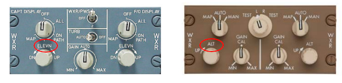
“Multi-ScanBuffering” radars are more sophisticated units with advanced CPU processors and come in two flavors: “Multi-Scan” and “Elevation”. The Elevation Type is the more advanced of the two. Both types utilize multiple scans at multiple tilt angles and save that data into a memory buffer for CPU processing. The primary distinction between the two types stem from how they post-process and display that buffered data, as well as the control inputs available. Below is an example control panel for a Multi-Scan buffering type.
The Multi-Scan Type will have Tilt Controls, which as stated previously, represents a commanded, reference tilt angle. This type of radar combines the multiple scan returns into a singular composite image that is displayed on the WX display. The composite display is essentially a layering of the multiple, angular ‘slices’.
The Elevation Type will not have any Tilt Controls, but will instead have a “Elevation” or “Altitude” control input as shown below.
The Elevation Type has more sophisticated algorithms and post-processing abilities, which allow the pilot to select a reference altitude, for which the CPU will assemble a final composite image that is relevant for the reference altitude as well as some distance above and below it. The following datarefs and commands allow you to configure the various modes available for Multi-Scan Buffering radars. Modes 0 & 1 are typical of the Multi-Scan Type and modes 2, 3 & 4 are typical of the Elevation Type. (Refer to Operating Mode Descriptions Above for each mode).
Weather radar multiscan for copilot display (ignores manual tilt dataref).
0 = Off,
1 = Combine scans (composite),
2 = Automatic altitude (on path),
3 = All Elevations,
4 = Selected Elevation (see datarefs below)
MULTISCAN MODE COMMANDS:
------------------------
sim/instruments/EFIS_wxr_multiscan_auto            Weather radar multiscan auto pilot
sim/instruments/EFIS_wxr_multiscan_on_path         Weather radar multiscan on path pilot
sim/instruments/EFIS_wxr_multiscan_all             Weather radar multiscan all elevations pilot
sim/instruments/EFIS_wxr_multiscan_elev            Weather radar multiscan one elevation pilot
sim/instruments/EFIS_wxr_multiscan_off             Weather radar multiscan off pilot
sim/instruments/EFIS_wxr_multiscan_auto_copilot    Weather radar multiscan auto copilot
sim/instruments/EFIS_wxr_multiscan_on_path_copilot Weather radar multiscan on path copilot
sim/instruments/EFIS_wxr_multiscan_all_copilot     Weather radar multiscan all elevations copilot
sim/instruments/EFIS_wxr_multiscan_elev_copilot    Weather radar multiscan one elevation copilot
sim/instruments/EFIS_wxr_multiscan_off_copilot     Weather radar multiscan off copilot
When in Mode 4 (selected elevation), you can use the following datarefs or commands to configure the selected reference elevation / altitude. Note that using these commands or writing to these datarefs will reset the tilt to 0º and display a flat horizontal slice at the selected altitude.
Dataref
Type
Description
sim/cockpit2/EFIS/EFIS_weather_alt
float
In Feet. Weather radar buffer selected altitude pilot's ND – used in computerized weather radar systems instead of tilt. Defaults to -1000 when angular tilt is used.
sim/cockpit2/EFIS/EFIS_weather_alt_copilot
float
In Feet. Weather radar buffer selected altitude copilot's ND – used in computerized weather radar systems instead of tilt. Defaults to -1000 when angular tilt is used.
RADAR ALT SELECTION COMMANDS
-------------------------------
sim/instruments/EFIS_wxr_alt_up                Weather radar alt up pilot
sim/instruments/EFIS_wxr_alt_down              Weather radar alt down pilot
sim/instruments/EFIS_wxr_alt_up_copilot        Weather radar alt up copilot
sim/instruments/EFIS_wxr_alt_down_copilot      Weather radar alt down copilot
Auxiliary Modes – Datarefs and Commands
Radar systems can have auxiliary sub-modes for various purposes to improve the display or detect windshear. The following datarefs and commands can be used to manage the radar sub-modes.
Dataref
Type
Description
sim/cockpit2/EFIS/EFIS_weather_stab
int (0 / 1)
Pitch/roll STABilization.
sim/cockpit2/EFIS/EFIS_weather_stab_copilot
int (0 / 1)
Pitch/roll STABilization, copilot side.
sim/cockpit2/EFIS/EFIS_weather_gcs
int (0 / 1)
Weather radar Ground Clutter Suppression.
sim/cockpit2/EFIS/EFIS_weather_gcs_copilot
int (0 / 1)
Ground Clutter suppression, copilot.
sim/cockpit2/EFIS/EFIS_weather_pws
int (0 / 1)
Predictive WindShear system.
sim/cockpit2/EFIS/EFIS_weather_pws_copilot
int (0 / 1)
Predictive WindShear system, copilot.
AUXILIARY MODE COMMANDS
-------------------------
sim/instruments/EFIS_wxr_stab_on              Weather radar stabilization on pilot
sim/instruments/EFIS_wxr_stab_off             Weather radar stabilization off pilot
sim/instruments/EFIS_wxr_stab_tog             Weather radar stabilization toggle pilot
sim/instruments/EFIS_wxr_stab_on_copilot      Weather radar stabilization on copilot
sim/instruments/EFIS_wxr_stab_off_copilot     Weather radar stabilization off copilot
sim/instruments/EFIS_wxr_stab_tog_copilot     Weather radar stabilization toggle copilot
sim/instruments/EFIS_wxr_gcs_on               Weather radar ground clutter supression on pilot
sim/instruments/EFIS_wxr_gcs_off              Weather radar ground clutter supression off pilot
sim/instruments/EFIS_wxr_gcs_tog              Weather radar ground clutter supression toggle pilot
sim/instruments/EFIS_wxr_gcs_on_copilot       Weather radar ground clutter supression on copilot
sim/instruments/EFIS_wxr_gcs_off_copilot      Weather radar ground clutter supression off copilot
sim/instruments/EFIS_wxr_gcs_tog_copilot      Weather radar ground clutter supression toggle copilot
sim/instruments/EFIS_wxr_pws_on               Weather radar predictive windshear on pilot
sim/instruments/EFIS_wxr_pws_off              Weather radar predictive windshear off pilot
sim/instruments/EFIS_wxr_pws_tog              Weather radar predictive windshear toggle pilot
sim/instruments/EFIS_wxr_pws_on_copilot       Weather radar predictive windshear on copilot
sim/instruments/EFIS_wxr_pws_off_copilot      Weather radar predictive windshear off copilot
sim/instruments/EFIS_wxr_pws_tog_copilot      Weather radar predictive windshear toggle copilot
X-Plane 12 can simulate both ice accumulation and window de-ice effects as well as rain drop/wiper visual effects on aircraft window surfaces. This article explains how to implement icing visual effects only. Rain effects are discussed in its own dedicated article, “Windshield Rain Effects”. This article assumes you are familiar with:
💡 NOTE: X-Plane 12.1+ introduces significant changes to the windshield ice and heat simulation from previous versions, which had many problems. Any RainGlass OBJs previously configured with THERMAL sources, and exporting from XP2B V4.3+ using an export target version prior to 12.1 will NOT have window heat functionality. The exporting of the legacy THERMAL_source directive have been removed for all XP version options prior to 12.1.
If you have exported out RainGlass OBJs with XP2B 4.3+ to support XP targets < 12.1, yet still desire to use the legacy THERMAL_source directive, then you will need to manually edit the OBJ and enter the directive and its parameters by hand. This directive and parameters are described further below for reference.
Enabling Ice Effects
Ice effects are automatically included on any window OBJs configured for Rain Effects. See the Rain Effects document for more info if you haven’t set up your RainGlass OBJs yet. When the conditions warrant, and in the absence of any window heat, the window will begin icing over uniformly at a rate dependent upon the conditions. X-Plane’s icing algorithm considers temperature, moisture, airflow and heating when calculating ice accumulation on RainGlass OBJs.
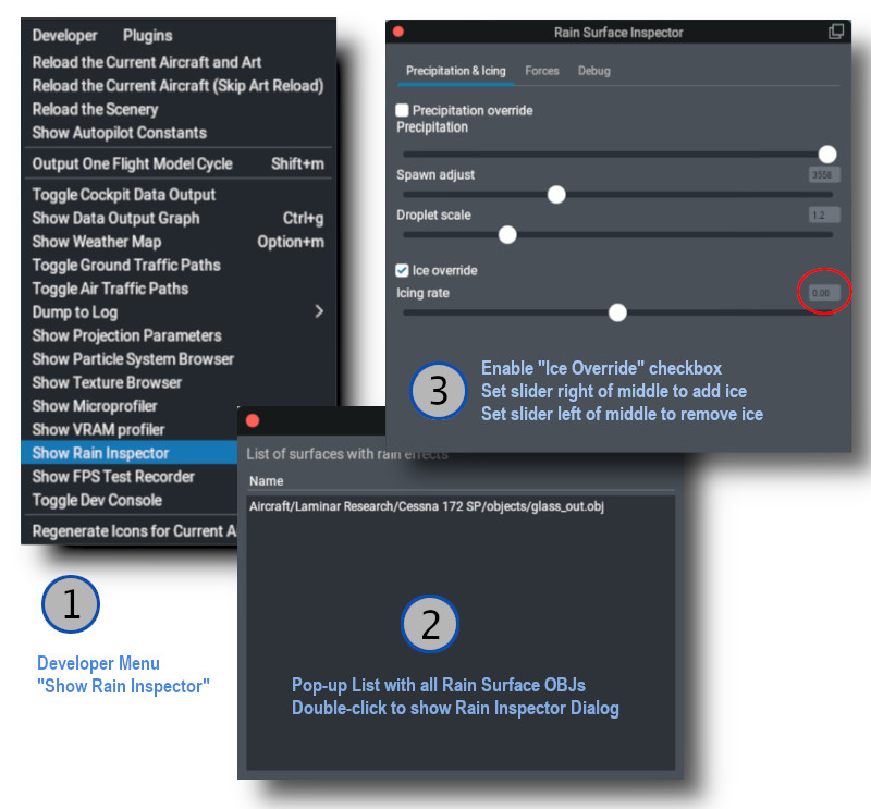
Icing Inspector Tool
The same tool that is used to debug / inspect Rain Effects is also used to debug / inspect icing effects, so you don’t have to configure X-Plane’s weather to test your work. The image below shows the sequence for use.
💡 NOTE: For the “Icing Rate” slider. The middle position is 0 (red circle below). The right side of the slider adds ice and the left side of the slider will remove ice. If you are wanting to test your thermal texture deicing effects quickly, you will probably want to move the slider to the right to add ice, and then return it to the middle zero position and then activate the window de-ice system to observe the effects of your thermal gradient texture.
Thermal Sources Gradient Texture
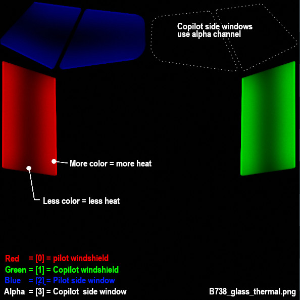
In reality, windshields are typically deiced using either resistance (electrical) heating elements, or by using hot air blowers. Both of these are examples of thermal sources. Thermal sources typically apply heat to specific areas of the windshield glass and the heat radiates out from that area across the windshield. This causes the ice to melt in a progressive pattern, melting nearest the heat source first and progressing from there. X-Plane models the progression of this heat flow via a 8-bit RGBA “thermal texture”, UV mapped to your RainGlass OBJ and using color gradients across the UV islands of the windows to model the movement of the heat.
X-Plane uses the four channels of the thermal texture to simulate up to four independent thermal sources. Most aircraft typically have only one or two thermal sources.
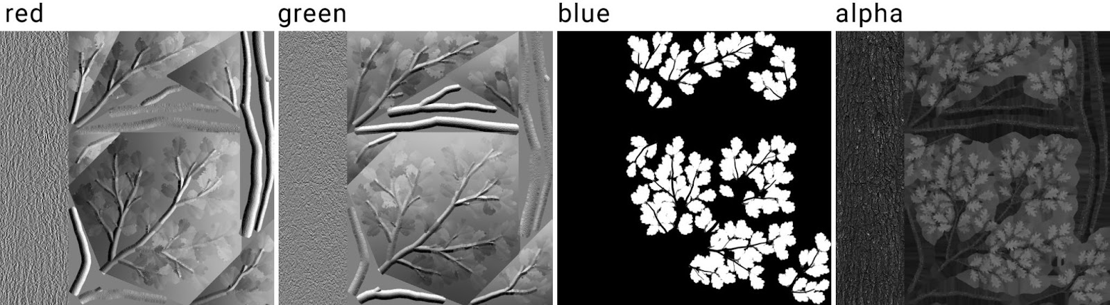
The image below shows an example texture where a fully saturated color pixel, i.e. 100% Red, Geen, Blue or Alpha(white) represents maximum heat flux and a fully black pixel represents zero heat flux. Note in the example below that there are no fully black pixels on the window glass because if there were, the window heat would not melt ice in these locations.
The gradient texture is quite straightforward, typically painted by hand using gradient tools in graphic apps like Photoshop or GIMP. Remember that a fully black alpha channel (when thermal source [3] is not used), will make your image transparent.
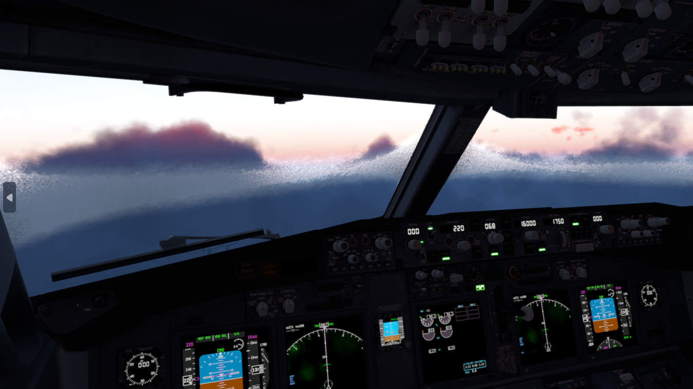
The image above illustrates how the thermal sources for the main windshields (Red and Green), are at the top and bottom of the windshields, and ice melts there first and then the heat moves towards the center of the window. In X-Plane the effect looks like so. For a hot-air blower fan configuration, you may have a radial type of gradient pattern, etc.
💡 TIP: Use a lower resolution THERMAL_texture to achieve better and more realistic looking heat propogation behaviours.
XPlane2Blender Settings
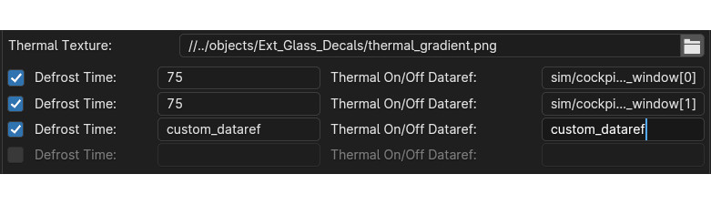
The XP2B settings for the thermal sources for window heat are found on Blender’s Scene tab in the collection settings (see image below). To configure your window heat, you enter the path to your thermal sources texture, presumably in the objects folder somewhere, and you enable however many thermal sources you need, up to 4 total.
For each thermal source you enable, you enter the Defrost time, in seconds. This field can be a fixed number or a dataref. This time represents how long, in seconds, a thermal source takes to fully deice a fully iced over window, assuming no ongoing ice accumulation. A shorter time represents more heating power. If you use a dataref, then you can alter this value at run time to simulate adjustable heating levels.
Next you enter the Thermal ON/OFF dataref. These datarefs, when 0, disable the window heat and when non-zero (usually 1), enable the window-heat. X-Plane have default datarefs for turning the window-heat ON/OFF for each source, which are listed further below.
The thermal settings in Blender will be exported to the OBJ GLOBAL settings in the form of two directives in the OBJ header section: one entry for the thermal texture file/path and one entry for each thermal source configured in Blender.
THERMAL_texture    path/to/texture/thermal_texture.pn;
THERMAL_source2   <index>    <rate_seconds or rate dataref>   <on/off dataref>
The exported windshield heat thermal parameters for the default B738, which uses four sources are shown below. Note that the ON/OFF datarefs are X-Plane’s status datarefs and not the window heat actuator/switch datarefs. The status datarefs take into account any system failures. You don’t want your window heat effects to be ON if the system is failed.
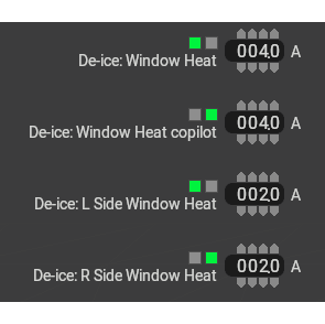
Power Consumption
You can configure the power consumption of each thermal source via PlaneMakers’s Standard Menu > Systems > Bus Loads Tab (the first one). When the status datarefs are 1, then X-Plane will add a current load to your electrical buses. These are fixed electrical loads only.
If you need to simulate a variable power window heat system and want to vary the power consumption of the thermal sources, then you will have to do so via plugin, adjusting your defrost time via dataref, calculating your power consumption and adding the load to a bus via sim/cockpit2/electrical/plugin_bus_load_amps[n]
Icing Commands and Datarefs
The following datarefs and commands are used with the Window heat / icing system.
        //  Actuator Datarefs (switch, button, whatever)
        sim/cockpit/switches/anti_ice_window_heat       // switch, 1st window
        sim/cockpit2/ice/ice_window_heat_on_window[N]   // switch, where N = 0-3

        // Actuator Commands
        sim/ice/window_heat_on                          // 1st window
        sim/ice/window_heat_off
        sim/ice/window_heat_toggle

        sim/ice/window2_heat_on                         // 2nd window
        sim/ice/window2_heat_off
        sim/ice/window2_heat_toggle

        sim/ice/window3_heat_on                         // 3rd window
        sim/ice/window3_heat_off
        sim/ice/window3_heat_toggle

        sim/ice/window4_heat_on                         // 4th window
        sim/ice/window4_heat_off
        sim/ice/window5_heat_toggle

        //  Status Datarefs.  Takes into account failures. e.g. can drive annuns
        sim/cockpit2/ice/ice_window_heat_on             // status, 1 window only
        sim/cockpit2/ice/ice_window_heat_running[N]     // status

        //  Failure State Datarefs
        sim/operation/failures/rel_ice_window_heat
        sim/operation/failures/rel_ice_window_heat_cop
        sim/operation/failures/rel_ice_window_heat_l_side
        sim/operation/failures/rel_ice_window_heat_r_side
Legacy Icing
It’s highly recommended to use the THERMAL_source2 directive with X-Plane 12.1.0 for any new aircraft development. The legacy THERMAL_source command still works in X-Plane 12.1.0, but the visual icing effects have inconsistencies with the X-Plane systems model with regards to how much ice X-Plane tracks on the windshield versus how much is visually rendered.
The syntax for the legacy THERMAL_source command is:
THERMAL_source <heat in ºC dataref> <on/off dataref>
…where the <heat in ºC dataref> is clamped between 5º and 20º C and then gets interpolated into a rate between 5 and 20 seconds.
💡 NOTE: Detail Textures were previously referred to as “DECALS”. The term DECAL is a legacy term. The OBJ directives: DECAL_PARAMS and NORMAL_DECAL_PARAMS are part of the OBJ specification and will not change; however, the term “Detail Textures (DTs)” are the official name for these specific texture types.
As of XP2B v4.3.3, the label “Decal” is used in the UI panels. Future versions of XP2B will adopt the label “Detail Texture” in lieu of “Decal”. Until such changes are integrated into XP2B, consider the terms interchangable in the meantime.
Introduction
Detail Textures, (DTs) are tileable, repeating textures that can be overlaid / mixed with either your OBJ albedo or normal textures. They were designed to add higher density textural detail without having to resort to large texel densities to capture those small details. Detail Textures were designed for use with ground textures but adapted for aircraft use; therefore, many of the XP2B DT configuration settings are not applicable for use in aircraft.
The image below shows DTs used to portray textured plastic and vinyl grain, where the albedo and DT texel densities are quite low, yet the DT overlay resolution is effectively higher because it is scaled down and tiled. By using less UV space on your albedo textures for these broadly colored areas, this frees up UV space to increase your texel density in other areas of your OBJ, or allow you to reduce the size of your albedo textures for more efficient VRAM usage.
Detail Texture Concepts
Refer to the image below:
An OBJ may have up to two DT Slots. Each slot may contain a ‘DT Albedo’ and a ‘DT Normal’ texture. Either DT in each slot may be used, one does not require the other. The example above only utilizes Normal DTs. The Albedo DT can have an alpha channel; however, the Normal DT ignores both the blue and alpha channels. Only the Red and Green channels of the Normal DT are utilized for normal/bump effects.
Each DT slot has its own scaling parameter. In the example below left, DT Slot 1 has a scale of 0.25 and DT Slot 2 has a scale of 0.5.
When using Albedo DTs, the color mixing with the Base Albedos is established by a graphics shader. There is no configurable ‘mixing mode’ such as “multiply / add / overlay”, and for Albedo DTs containing high saturation hues, the results can be unpredictable. Albedo DTs for aircraft use are best suited for adding lower saturation hues.
DTs are tiled orthogonally, there is no provision to rotate the tiled pattern.
An optional Red / Green channel Modulator Texture (MT) may be utilized as a mask, to control where DT1 and DT2 are applied to the Base Albedo texture.
A Base Albedo texture is required to use Albedo DTs and a Base Normal Texture is required to use Normal DTs.
The XPlane2Blender settings for Detail Textures (DTs) are found on the Scene Properties Tab as shown below. Additional fields will appear once you enter the DT filenames. The image below shows the XP2B UI widgets for Albedo DT and one Normal DT. The good news is that for aircraft use, we do not need too many of these options. The highlighted areas in green are the only fields you need to be concerned with for aircraft use. The others fields are used for scenery development and ground texture DTs. Each field is as follows:
SCALE: The scale isn’t exactly a scale factor in the typical sense, but rather the “number of tiles” along the edge of the albedo, ergo it is the inverse of the scaling factor. In the example above left, the scale would be 4. This field should be a value ≥ 2. One tile makes no sense as you could just mix the textures together in Photoshop.
RGB Decal Modulator Strength: This is most easily described as a type of opacity or ‘strengh of effect’ value. A value of 1 mixes the DTs with the Base Albedo with full strength. Lower values reduce the effect of the DTs. (Example further below). A value of zero effectively negates the DT effect.
Modulator Strength: Same as above, but for the DT Normal Texture.
Modulator Texture: A Red/Green channel texture to use as a mask for DTs 1 and 2. The red channel of the Modulator Texture will control where DT1 is applied and the green channel controls where DT2 is applied. The Red and Green channels may be mixed to apply both DT1 and DT2 to the same area of the texture. If no Modulator Texture is specified, then the DTs will be applied uniformly over the entire Base Albedo.
Examples
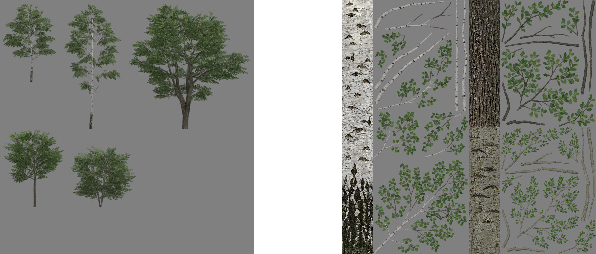
The best way to illustrate the use of Detail Textures are with examples. We are going to start simple and get progressively more complex. We will be using the following Objects and Textures below in our example. We have two Albedo DTs and 3 Normal DTs to work with, in addition to our Base Albedo and Normal textures.
This is what it looks like in X-Plane without any Detail Textures applied:
Normal Detail Textures
We first begin with normal textures, because they are the most likely application with aircraft. We apply a Leather grain normal texture (256px) by specifying leather_NML.png as Detail Texture 1, setting the Modulator Strength to 1 and arbitrarily set the scale/tiles to 50. The results look like so.
In the above image, note that the effect is applied over the entire OBJ, including the knob because no modulator texture was specified to mask areas of the texture. We will now specify a modulator texture to limit the leather grain effect to just the gauge surround using the RED channel, since this is a Slot 1 detail texture.
In the image below, the settings are the same as above, except for the addition of the Modulator Texture, “decal_mask.png”. Some of the gauge surround now have DT Effects (yellow mask) and some areas have no DT effects (black areas of mask = no effects). Note that YELLOW is equal parts RED and GREEN so any UV islands mapped to yellow will receive both DT1 and DT2 effects; however, because no DT2 has been specified yet, only DT1 shows up on the gauge surround. Lets add a second Normal DT texture to add some noise on top of the leather grain.
In the image below, we have added a second Normal Map Decal 2 with the 3 settings in XP2B circled in red. Because this is DT2, it is masked with the GREEN color channel. Since the knob UV is masked with GREEN, it receives the noise DT, but not the leather DT. The leather DT is indeed on the gauge surround, but it is overpowered by the noise DT effect. Lets reduce the Modulator Strength of the Noise DT a bit and scale up the leather DT slightly so we can see both effects on the gauge surround due to the YELLOW mask.
In the image below, you can see how the gauge surround now has both leather and noise normal effects. Also note how the modulator Strength reduces the effect of the Noise DT. Once you have specified your Normal DTs, simply adjust the Scale and Modulator Strength values to tweak the effect. Lets wrap up this section on Normal DTs with one last example. We’ll swap out the noise DT for the knurl_NML.png DT and set the Modulator Strength back to 1. The result is shown in the 2nd image below.
Albedo Detail Textures
Albedo textures are configured in the exact same way as the Normal DTs. Though there are more UI Widgets available for the Albedo DTs (for scenery textures), for aircraft you still only work with the same two input types as for Normal DTs, i.e. the Scale value and the RGB Decal Modulator Strength value.
As mentioned above, the color mixing of the Albedo DT with the Base Albedo is non-intuitive. The example below left shows a low-contrast noise_ALB.png added to the flat plate to add some grayscale noise color. The middle image shows the same flat plate, but with the noise Normal DT added in also. The right image shows a second, high contrast Albedo DT added, dots_ALB.png and illustrates how the color mixing of the Albedo DT with the Base Albedo yields a not so intuitive result that differs based on the pixels of the Base Albedo. (See original texture, dots_ALB.png texture above). Albedo DTs are best for applying more saturated, low-contrast colors, such as grime and dirt or to disrupt a bit of color uniformity.
OBJ Output
The image below shows the typical entries in the OBJ header for Detail Textures as XP2B exports the data. The order of the entries in the OBJ determines whether or not a Detail Texture is in Slot 1 or 2, and therefore, which will be affected by the RED and GREEN channels if a modulator texture is used. The XPlane2Blender UI references DTs 1 and 2, but this is semantic. If you specify DTs in XP2B in the DT2 slots, but leave the DT1 slots empty, then only one slot will be used in the OBJ and as such, any modulator ‘masking’ would be controlled by the RED channel. Best practice in XP2B is to simply use the DTs in order, i.e. DT1, then DT2 if required.
Summary Review
Take advantage of why Detail Textures exist, i.e. save VRAM by using smaller textures where you are able. If you use a Detail Texture with a scale factor (tiling) of 1, there is no benefit.
Keep texel densities the same for UV islands that use the same Detail Textures so the effect is consistent across all meshes using it.
Use the Detail Texture Slots in the order they appear in XP2B, i.e. DT1, then DT2
To recap, the Modulator Texture is for masking, the RED channel is the mask for Detail Texture 1 and the GREEN channel is the mask for Detail Texture 2.
X-Plane 12 can simulate both rain drop/wiper visual effects as well as icing and window heat effects on aircraft window surfaces. This article explains how to implement and calibrate rain effects only. Icing effects are discussed in its own dedicated article, “Windshield Ice Effects”. This article assumes you are familiar with:
The 3D OBJs to receive rain effects should only contain polygons for surfaces with rain effects. Do not include opaque or non-rain-effects polygons as part of your rain-glass objects.
You should expect to use two separate OBJs to represent your rain glass: one OBJ with outward facing normals and another OBJ with inward (cockpit/cabin) facing normals. Best practice is to name these two OBJs as follows for clarity reasons:
Each individual window should to be a continuous, manifold mesh in 3D with no UV seams, so that when UV unwrapped, the resulting UV island mesh is also continuous. Do not split up a singular window into multiple UV islands.
No UV island of any one window should overlap another on the texture. UV islands should have consistent texel densities between them and minimal warping for consistent rain drop sizes.
Any transparent meshes inside the aircraft, (typically translucent sun-visors) where you need to see the rain effects through these meshes, should be part of the inside_reflector object; however, the draw-order of the meshes within that OBJ may need to be configured (more below).
While you CAN use multiple OBJs set to Outside Rain Glass, this is not recommended. You should endeavor to use one OBJ for all external glass with rain effects and a second OBJ for all the inside (reflector) facing glass.
Enabling Rain Effects on OBJs
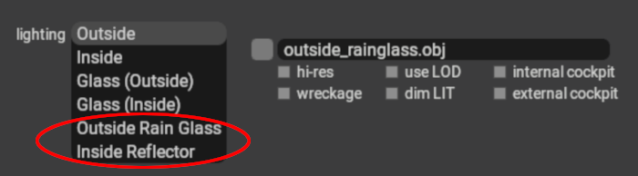
Rain effects can be enabled on your window OBJs by setting their lighting mode in PlaneMaker to either Outside Rain Glass or Inside Reflector. Use Outside Rain Glass for your OBJ with outward facing normals and use Inside Reflector for any windows (or visors) with inside/cockpit/cabin facing normals.
These two OBJ lighting settings are complementary and intended to be used together. If not utilized together, then inconsistent rain effects in various X-Plane views may result. X-Plane will simulate raindrops on these OBJ meshes, including the effects of gravity and aerodynamic forces.
UV Considerations for Rain Glass
To avoid differing raindrop sizes on your individual windows, ensure that the texel density of your UV islands are consistent.
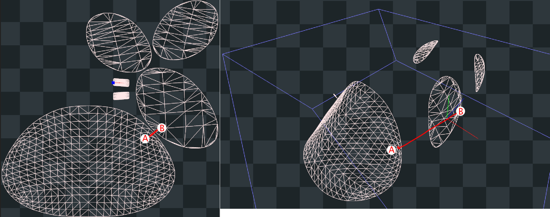
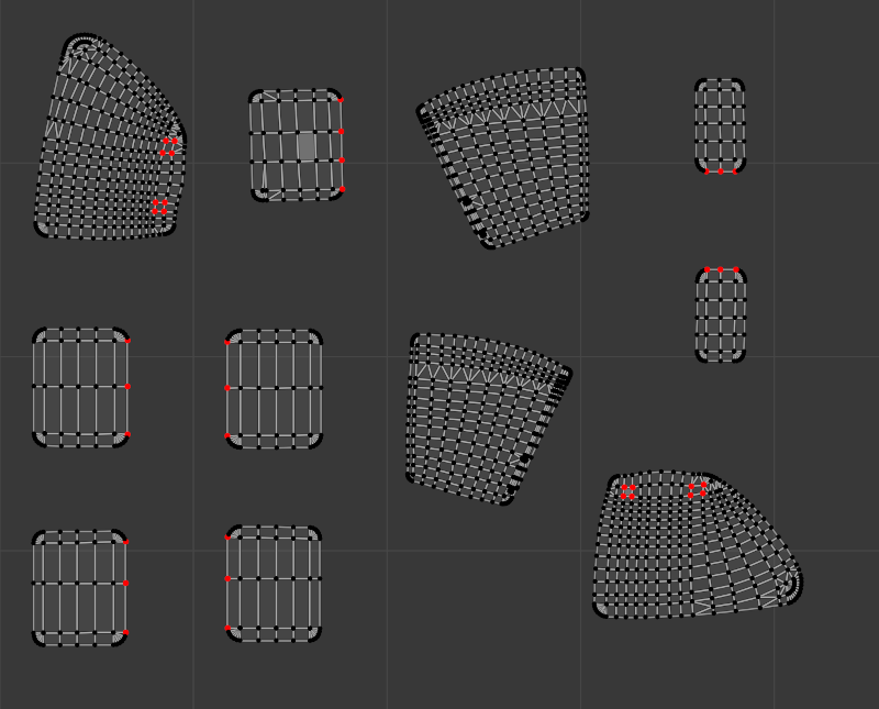
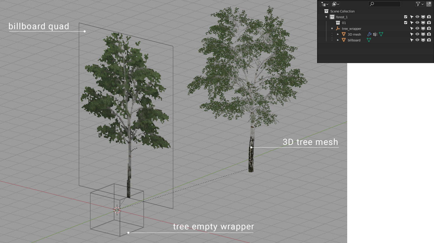
Regarding UV island packing, each flight loop, the rain algorithm calculates the velocity, direction and momentum of the raindrop in 3D space and then animates its translation on the 2D texture accordingly for the next flight loop. The algorithm knows when a raindrop is within the bounds of a UV island, so when a raindrop has been calculated to move outside of any UV island, then the raindrop ceases to exist. If your UV islands are packed close enough together, then the speed and momentum of the raindrop may be enough where the raindrop “jumps” from one UV island to an adjacent one in 2D space during one flight loop calculation. This effect is illustrated in the screenshots below on the default Lancair Evolution.
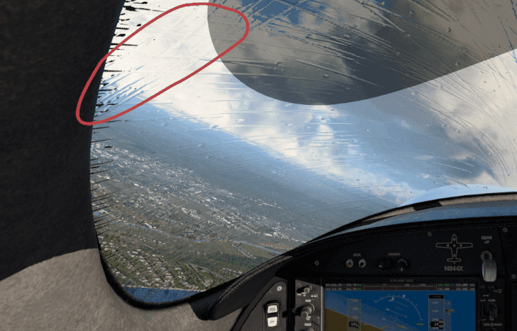
On the UV map (left side), the window uv islands are placed very close together, but the physical 3D locations of the window elements (right side) are not that close together, so in reality, a raindrop would not instantly jump from point A to point B as shown below, yet because the UV islands are close together, the algorithm may animate the raindrop as if this is what happened. If your UV islands are not aligned in a natural way, then a “jumping” raindrop could appear to change directions as its momentum carries it into the adjacent UV island, but with the direction vector from the previous UV island. The red circle in the image further below shows the undesired result of such a situation.
There are three ways to avoid this unwanted effect:
1. Use TRIS_break Directive (12.1+ only)
This is the preferred method for projects supporting X-Plane 12.1+ only. It allows for maximum UV island packing efficiency. If using this method, then each individual window should be separated to be its own mesh object in Blender. If using XPlane2Blender V4.3+, then on each window mesh, enable the “Rain Cannot Escape” checkbox_**.**_ The TRIS_break directive will then be applied to each window mesh. The image below shows the checkbox option and the typical results in the OBJ file.
The TRIS_break directive is a ‘separator’ between TRIS commands and does not need to exist both before and after a TRIS entry in the OBJ file; however, Xplane2Blender may put extra TRIS_break directives before and after some TRIS commands, which is fine. If you are manually editing the OBJ file, just know that a single entry between your rain glass TRIS is all that is required to prevent ‘raindrop jumping’ between those TRIS groups.
2. Align UVs in a Natural Way
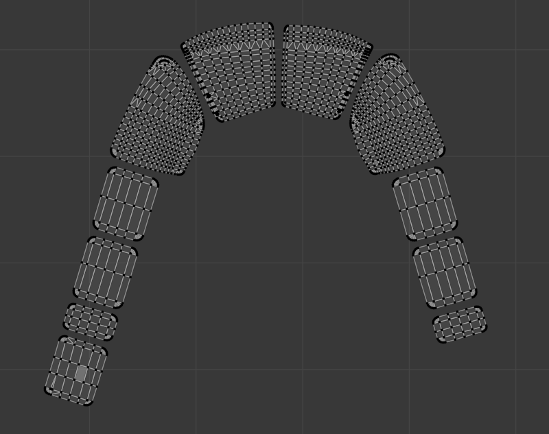
If you want to pack your UV islands tight, get good visual results, and still support X-Plane versions prior to 12.1, then you can align your UV islands so that if a raindrop is moving fast enough that it migrates from one UV island to the next in a single flight loop, then it will be moving in a consistent direction between the UV islands. The example below shows how such UV islands might be aligned. If using this method, then each window does not need to be separated into its own mesh object, all windows can be part of a single Blender mesh object. This method is not recommended for large rainglass texture sizes! as it wastes too much textures space and VRAM. The better solution for pre 12.1 rainglass support is to pack your UV islands just tight enough to avoid raindrop “jumps” (method 3 below)
3. Spread out your UV Islands
The third option is to spread out your UV islands as required, orienting each island any way you like as long as they’re just far enough apart where a raindrop is unlikely to translate from one UV island to another in one flight loop calculation. As raindrops move outside a UV island, they cease to exist. Again, this method wastes some texture space similar to method 2 above, but not as much. As with option 2 though, the windows do not need to be separated into their own mesh objects. This is the better method if you want to support XP version before 12.1.
Windshield Friction (12.1+ only)
Different windshields might have different coatings applied to them to affect how rain interacts with them. For example, on aircraft with blowers, the windshield tends to be coated with a highly rain repellant material to avoid rain drops accumulating or streaking over them. Likewise, some aircraft also have the option to apply rain repellant during the flight to decrease glass friction. Starting with X-Plane 12.1.0, this can be modelled using the following GLOBAL directive in the OBJ header section.
RAIN_friction <some/dataref/and/default_is_1>
The dataref lets you adjust the friction dynamically at runtime, although most aircraft will probably just use a fixed value as this is not a common option on aircraft glass. Decreasing the value will decrease glass friction and also decrease the likelihood of rain drops becoming streaks.
Rain Drop Size / Scale
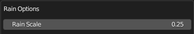
X-Plane creates rain drops with a default, unitless size of “1” and depending on the texel resolution of your UV islands, the rain drops may need to be scaled up or down for your application to look more plausible. The scale of the raindrops may be altered to be bigger or smaller via an OBJ Global Directive, “RAIN_scale”. This scaling factor can be set via the Collection Properties Panel. This value is typically set after testing in X-Plane using the Rain Inspector Tool described next.
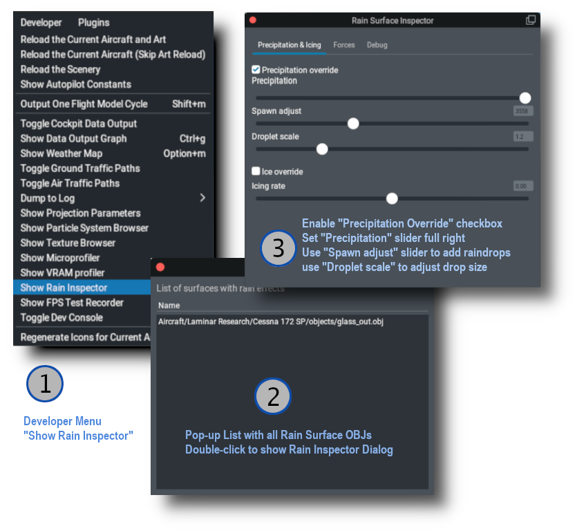
Rain Inspector Tool
X-Plane has a tool to debug Rain Effects in sim. This tool was developed for internal Laminar use but proved useful enough to make available to the public. Being an internal tool, it has several settings you will not need to be concerned with. This tool allows for quick testing of the rain effects without having to change X-Plane’s weather settings. The image below shows the sequence for use. If you have configured your OBJs to be rain glass/inside_reflector, you will see the rain effects in X-Plane as you make adjustments to the Spawn and Scale sliders. Note that its typical to run your test on the Outside Rain Glass OBJ only since that is the only surface exposed to the rain.
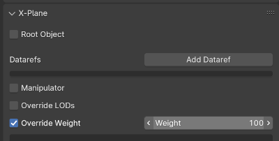
Be sure you check the rain effects from both inside and outside the aircraft. If you have any translucent sun visors, then make sure you can see raindrops through those as well. If you cannot, then make sure your sun-visor meshes are part of your Inside reflector OBJ and also that your sun-visor meshes have been configured to draw last within the OBJ by using XPlane2Blender’s “override weight” option on the object property Tab as shown below. Mesh objects assigned a weight value will draw in the order of their Weight values, with the highest weight value mesh objects drawing last.
3D Windshield Wiper Effects
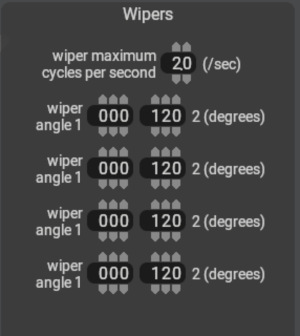
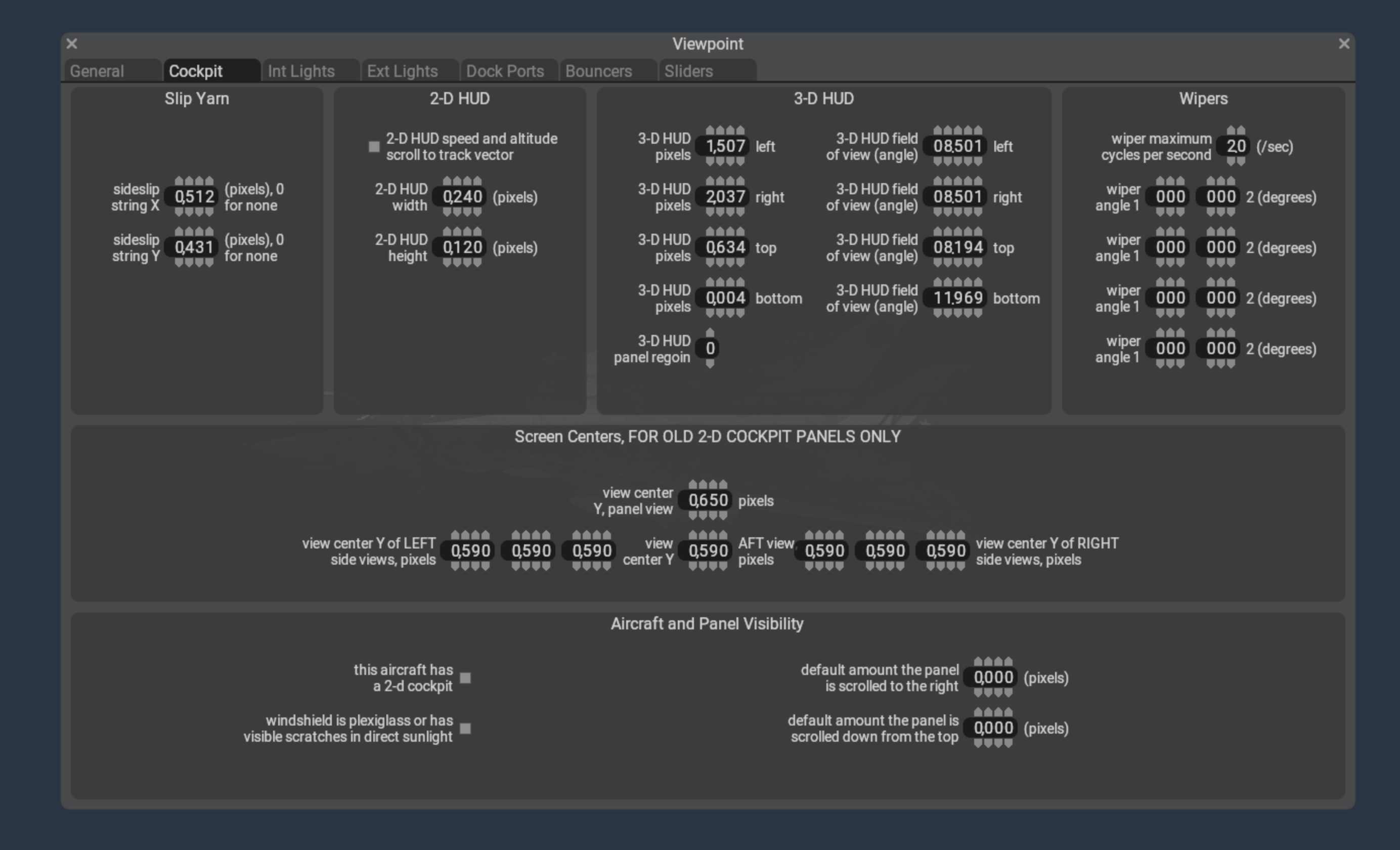
If your aircraft have 3D windshield wipers, you will first need to configure the periodic timing of the wipers in PlaneMaker via the Standard Menu > Viewpoint > Cockpit Tab > Wipers panel as shown in the example screenshot below.
In this panel, you specify the limit angles of the wiper travel (usually 0º to some max valueº) and their oscillation frequency. These fields establish the range of values of the four wiper angle datarefs below, which can be used to drive your 3D wiper animations as well as the 2D wiper effects.
// Dataref to turn on the wipers
sim/cockpit2/switches/wiper_speed_switch    // 0 = park,    1 = 25%speed,   2 = 50%speed,    3 = 100%speed.

// Datarefs for the Instantaneous Angle of the wiper arms
sim/flightmodel2/misc/wiper_angle_deg[0]
sim/flightmodel2/misc/wiper_angle_deg[1]
sim/flightmodel2/misc/wiper_angle_deg[2]
sim/flightmodel2/misc/wiper_angle_deg[3]
Since the raindrop animations happen in 2D texture space, and windshield wiper animations exist separately in 3D space, then we need a way for the 2D rain algorithm to know where your 3D wiper blades are on the window so the effects are in sync. You don’t want the 2D rain wiper algorithm wiping away raindrops behind or ahead of your 3D wiper blade, so timing the 2D effect with your 3D animation is critical.
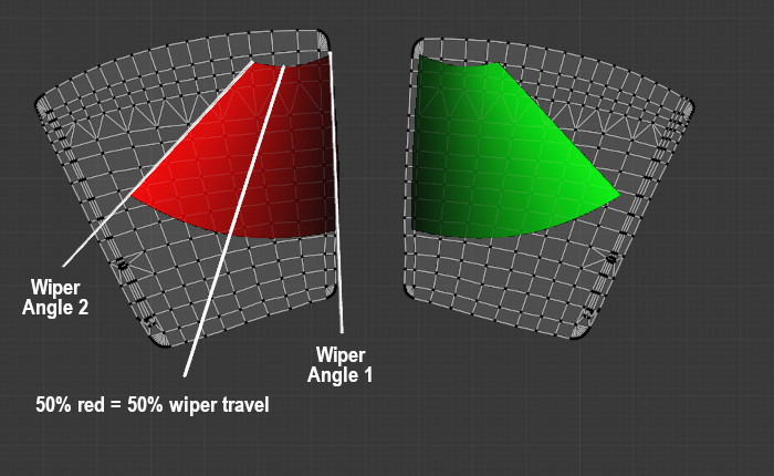
The 2D wiper position reconciles with the 3D position through the use of a dedicated “wiper gradient texture”, with colored gradient regions that represent the area swept by the 3D wiper blades across the UV islands. The color black represents one extreme position of your wiper travel (0% / wiper angle 1) and a fully saturated color channel (100% red / green / blue / alpha(white)) represents the other extreme position of your wiper travel (wiper angle 2). The example below shows how these swept gradient regions overlay the UV islands of windows as well as how the gradient values represents wiper travel.
Because we use a single image with four channels (RGBA) to contain the wiper data, this means we can simulate up to four independently controlled wiper blades per OBJ, but most of the time there’s just one or two. The image below shows what a typical wiper texture looks like for two independently controlled wipers where RED = wiper 1, GREEN = wiper 2. (BLUE = wiper 3, Alpha = Wiper 4, neither of which are used below). Note that if both wipers were controlled together by a single dataref (wiper 1), then both wiper gradients would be RED.
If your windshield wiper animation is completely linear, i.e. you only have two keyframes at the extreme positions, then the gradient texture would also be completely linear along its arc and you might could paint this texture by hand with some deft software ninja skills, but its not always as easy as it may appear and getting the gradient exactly right so the wiper effect matches the 3D wiper position can be a challenge. Fortunately, XPlane2Blender has a solution for us! The “Bake Wiper Gradient Texture” tool.
Wiper Gradient Texture Baking
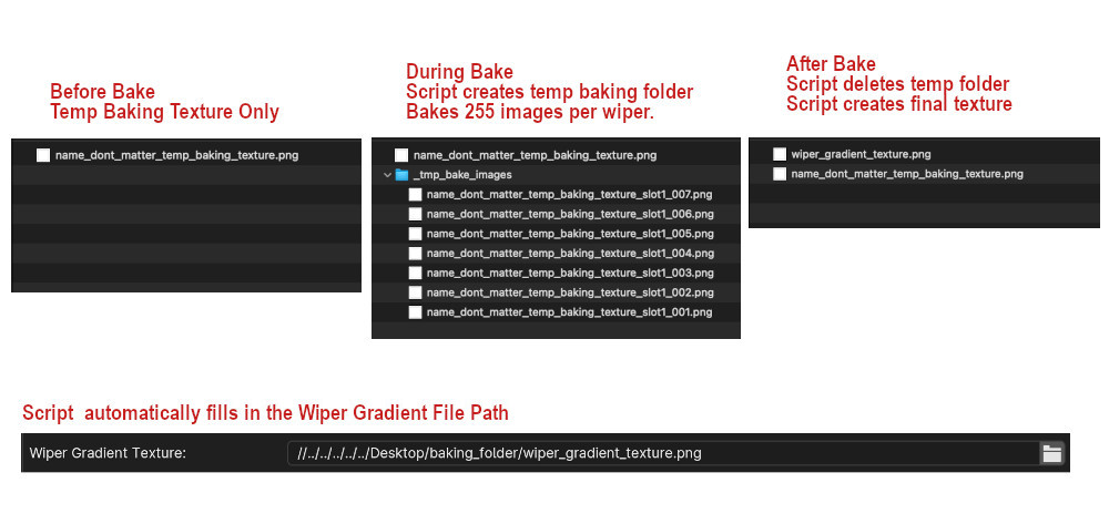
This tool will automatically create your Gradient Wiper Texture for you by using your 3d animation to generate the 2D wiper texture. In general, you’ll create a temporary ‘baking texture’, input/set multiple parameters in Blender, begin the bake, and during the bake process, the script will create a temporary folder and bake 255 temporary images per wiper. After that baking step, the script will then use those temporary images to create the final wiper texture, save it and delete the temporary folder. The baking process can take a while depending upon your machine capabilities, bake settings and texel densities. The single wiper example shown below was done on a Mac M1 laptop and took approximately 12 minutes total with a conservative texel density. Higher texel densities will increase bake times.
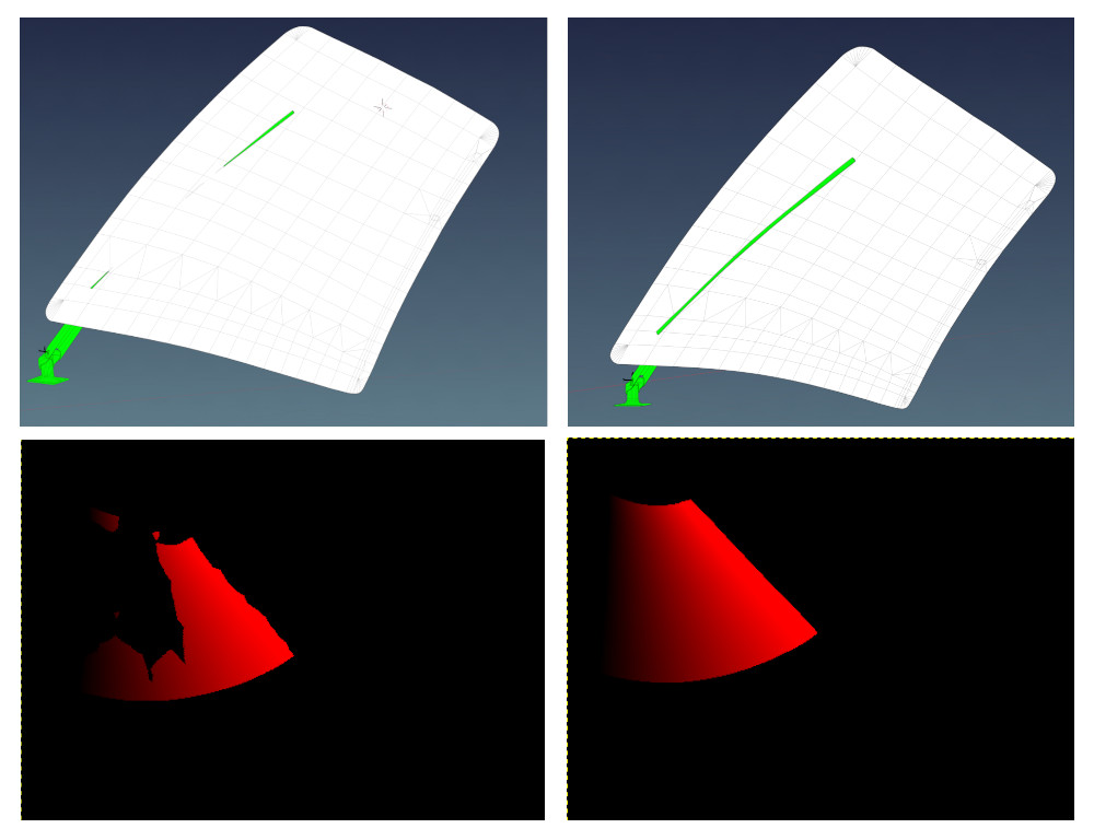
💡 IMPORTANT: For usable results, the wiper blade and windshield need to be in “collision contact” throughout the animation, i.e. the blade penetrates THROUGH the windshield mesh. If not, you may end up with areas on the UV island that are not calculated properly and you will get blotchy results. The image below shows the difference in results with partial intersecting geometry (left side) vs. fully intersecting geometry (right side). Its common to duplicate a blade temporarily and reshape / extend it through the windshield just for the gradient bake and then discard it after.
There’s a lot of steps in the baking process, so we’ll just dive right in via a step-by-step checklist:
Make sure ‘Cycles’ is the active renderer. It will not work with Eevee or Workbench.
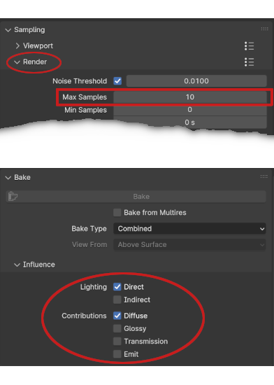
Set your Cycles Render samples (not Viewport) to a low number, like 10, and set your Lighting and Contributions check boxes as shown below. (Blender 4.1 shown). This will reduce baking time.
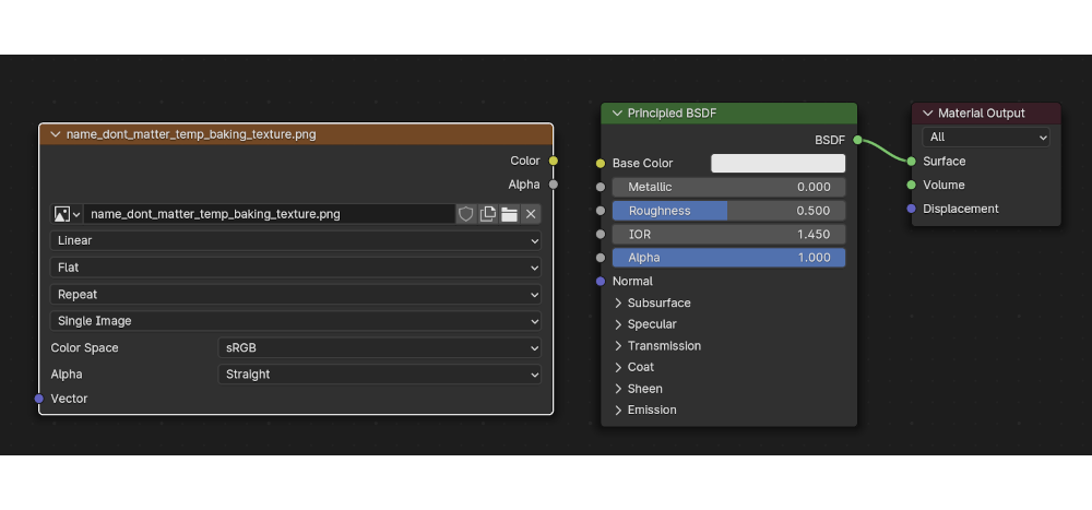
A four channel (RGBA), 8-bit per channel (32 total) “temporarybaking texture” must exist beforehand. Create, name and save an empty PNG the same size as your final texture, any filename will work. If you use Blender’s Image>New menu to create the image, do NOT select the ‘32-bit Float’ checkbox option, this results in 32-bits per channel, not 8 and will prevent the bake.
You can put this temporary texture anywhere you like for the bake, but we recommend putting it in the same location where you normally keep your other OBJ textures because the script will automatically create the final wiper gradient texture in this same location AND automatically enter the file path in the “Wiper Gradient Texture” text field for you (overwriting any existing entry). If you move the wiper gradient texture to some other final location after the bake, you will need to adjust the file path so it gets written to the OBJ header correctly.
Add an Image Texture Node to your rainglass material, and select the temporary baking texture you created in the previous step. The wiper script leverages Blender’s baking workflow and gets the file path to the baking texture from this image texture node. Unlike a regular Blender bake however, the image texture node need NOT be selected to bake, but does not matter if it is. Below is an example of an image node with the temp baking texture selected.
Animate your wiper motion over 255 frames (required). You can begin at any keyframe ≥ 1, but your last keyframe needs to be (Begin keyframe + 254). So if you begin your animation at keyframe 1, then your last keyframe will be 255. If you begin at keyframe 16, your last keyframe is 270, etc. The baking UI dialog allows you to specify the first keyframe value and Xplane2Blender will add 254 to it. The default begin keyframe is 1, we recommend you stick with that. You can use as many intermediate keyframes as is required for your animation. TIP: If you have already animated your wipers, but not over 255 frames, then note that Blender’s scale(S) command works on keyframes! Set the animation playhead on your first keyframe, select all keyframes for your wipers, hit ‘S’ and simply scale all your keyframes until the last one is 254 frames after the first one.
If you want to bake all wiper regions at the same time, then combine all window mesh objects that have wiper effects into a single mesh object (CTRL-J) for the bake. Give the mesh object (in the outliner) a unique name, e.g. wiper_windows. After the bake, you can separate out the mesh islands if need be, for example if you’re using TRIS_break option on each mesh object. You can also bake each wiper region separately if you want to and combine the images manually, i.e. you need to rebake one window only.
To shorten the bake time further, you can separate out the wiper BLADE mesh only (the part that touches the window). The fewer polygons involved in the calculation, the better. Give the wiper mesh objects that intersect the windows unique names (in the outliner) such as:
right_wiper_blade
left_wiper_blade
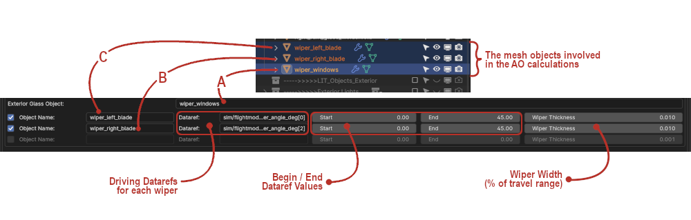
Now its time to enter all the pertinent data into the Rain Options panel (Scene Tab Collection Settings). Note that if your “Wiper Texture Gradient” text field is empty (the script will fill it in after the bake), then the wiper UI elements may appear grayed out; however, this is simply visual and you can still enter information in them. You will be manually entering mesh object names (from the outliner) into the Wiper settings text fields. If you misspell the name, the script will let you know with an error pop-up when you try to bake. In the example screenshot below, Item A is the Exterior Glass Object with wiper effects. Item B is a wiper blade mesh and Item C is a second wiper blade mesh. These fields tell the script which mesh objects to include in the baking process. If you have more wiper blades, just enable the bottom checkbox to enter their data. The example below will bake two wiper gradient regions to the RED and GREEN channels of the gradient texture.
NOTE: Each time you enable a checkbox, a new one will appear, up to 4 total. In the Object Name text box, enter the name of the Wiper Blade Mesh Object. Confirm name in Outliner. The first wiper will be Wiper 1 (red), the second Wiper 2 (green), etc, etc.
Enter the name of the driving datarefs for each wiper and keyframe values. This data will get written to the OBJ file. Common datarefs are:
sim/flightmodel2/misc/wiper_angle_deg[0]
sim/flightmodel2/misc/wiper_angle_deg[1]
The following two items are required in order for the Bake Wiper Texture Gradient button to activate.
The collection with the rainglass meshes must be enabled for export on Blender’s Scene Tab.
The collection with the raingless meshes must be selected in the outliner.
Time to Bake! On Blender’s Render Properties Tab, and with the above two criteria met, the “Bake Wiper Gradient Texture” button should now be active. Press the button to begin the bake. The image below shows the sequence of the Gradient Texture Baking Process.
A few things to note about the bake process:
During the bake, you will not see any animation in the 3D viewport. The wipers will not move. Blender is essentially “frozen” with no progress indicator, so don’t plan on doing any work in Blender while the bake is going on.
You can monitor the progress by observing the contents of the ‘__tmp_bake_images_’ folder, which will be growing with files as the 255 images (per wiper) are baked. Do expect 10+ minutes per wiper channel.
Once all images are baked, there will be a period of time with no apparent activity as the script calculates and assembles the final gradient image.
When complete, the temporary folder will be gone, the “wiper_gradient_texture.png” file will be in the folder and Blender will be functional again.
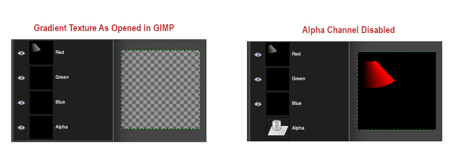
💡 NOTE: The script writes to all four image channels (RGBA) regardless of how many wipers are configured. If baking less than 4 wipers, the alpha channel will be completely black and as such, the RGB channels will be transparent when you open the image; however, the color information for the baked channels is present as can be seen below. Disabling the alpha channel will reveal the RGB channels.
Exporting and GLOBAL Settings
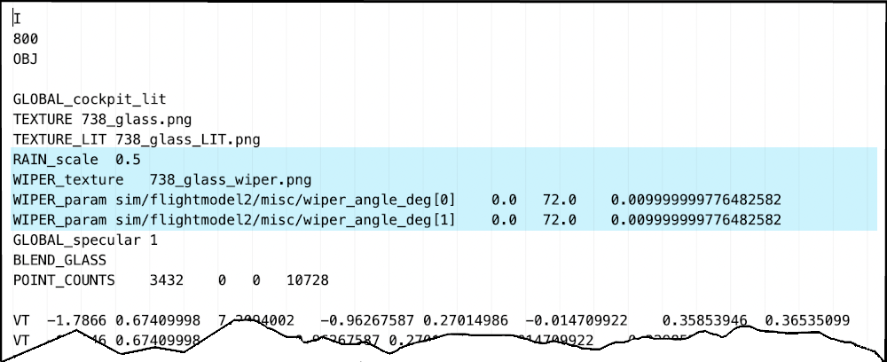
After exporting your rainglass object, the rain settings will be present in the GLOBAL properties of the OBJ as shown below. The default 737 example below has two independently controlled wipers, a custom rain scale and one wiper gradient texture. Remember that the wiper baking script will auto-name the baked texture, “wiper_gradient_texture.png”, but you can rename it to anything you like. If you do rename it, then make sure you also change the filename in XPlane2Blender’s “w_iper gradient texture_” text input box. Its good practice to check the exported OBJ to make sure all the settings and filepath are as expected.
The following is a download link for the sources for the Laminar Research default Boeing 737-800 sound bank. The project requires FMOD Studio 2.02.19 or greater. You can download FMOD Studio from the FMOD site.
You can use this project to learn how the sound for the 737 was created and experiment using the Live Reload feature. As the License below explains, you can only use it for learning purposes and you may not redistribute any part of it.
License
LICENSE AGREEMENT: B737 FMOD PROJECT AND SOURCE AUDIO CONTENT

This B737 FMOD Project and Source Audio Content License Agreement
(the "Agreement") is a legal agreement between you and Laminar Research.
By downloading, viewing, and in any way using this B737 FMOD project file
(the "PROJECT"), you agree to be bound by the terms of this Agreement.
If you do not agree with this Agreement, do not use this PROJECT.
All rights not expressly granted to you here are reserved by Laminar
Research. Upon acceptance of this Agreement, Laminar Research grants a license
to you to use this PROJECT expressly for educational or personal purposes only.
This license is granted worldwide and in perpetuity.

This Agreement includes license terms for:

a) The PROJECT, and any .bank files built thereof (altogether, the "FMOD
CONTENT"), and

b) The included .wav sound files (altogether, the "SOURCE AUDIO").

GRANT OF LICENSE:

1. FMOD CONTENT:

    You may modify, remix, redesign, and build upon the FMOD CONTENT.

    You may NOT share the FMOD CONTENT, original or otherwise modified.

    You may NOT broadcast video of the FMOD CONTENT, original or otherwise
    modified.

    You may NOT use the FMOD CONTENT for commercial or non-commercial purposes.

    You may NOT share, copy, or otherwise redistribute the FMOD CONTENT
    or any part of it.

2. SOURCE AUDIO:

    All SOURCE AUDIO is owned by Laminar Research.

    You may NOT share, copy, or otherwise redistribute the SOURCE AUDIO.

    You may NOT use the SOURCE AUDIO for any commercial or non-commercial
    purposes.

    You may modify, remix, redesign, and build upon the SOURCE AUDIO, provided
    it is strictly for PERSONAL use.


If you have any questions about this Agreement, please contact Daniela
Rodríguez Careri at <daniela@x-plane.com>.
Starting X-Plane 12.00 you can customize the airport ground vehicles. Since those are part of the APT.dat defined scenery, they are loaded early and separately from DSF scenery, and cannot be replaced via a EXPORT override on the library.txt like other library objects.
This feature allows you to make vehicles that you can include either locally in a custom scenery or as a part of a library to use in one or many of your airports. Bear in mind, though, that the custom vehicles have to be placed manually at each parking location. There’s no global replacement.
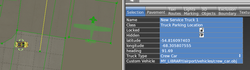
Each “Service vehicle parking location” in WED now has a “Custom vehicle” field where you specify your replacement object. The object itself will be moved around at the same speeds as the selected service truck, for the same purpose (crew car, GPU, fuel truck etc), i.e. the behavior itself is not customizable.
All components of the object (sounds, driver object etc) can be customized by the library author by providing suitably named components to go along with the vehicle object.
How to
Create your vehicle 3D model with animations. The datarefs available for animations and sound are those under sim/graphics/animation/ground_traffic/ (see the Dataref list)
On the SND file (see SND file specification) use start/end conditions according to the datarefs mentioned above. You can also use those datarefs as parameters inside FMOD Studio to modulate the events.
Ensure the events are assigned to the Master Bank androuted to the Exterior Processed > Environment bus.
If you need to apply signal processing (reverb, EQ, etc) to the sounds, don’t apply them to the Environment bus itself because they will be overriden by the corresponding aircraft bus processing. Instead, create a subgroup under Environment to do so.
Expose the object on the scenery or library library.txt (see library.txt specification) so WED can use it, via a EXPORT directive. For example
In WED, place a parking location of the kind of vehicle you want to replace (fuel truck, catering, etc) and under the “Custom vehicle” field, enter the virtual path to your custom vehicle from your library. For example
1 – As a first step, you need to put down an exterior facade. You can use any of the facades from lib/airport/hangars/flat/xxx.fac. Make sure the shape is orthogonal (CTRL + Q).
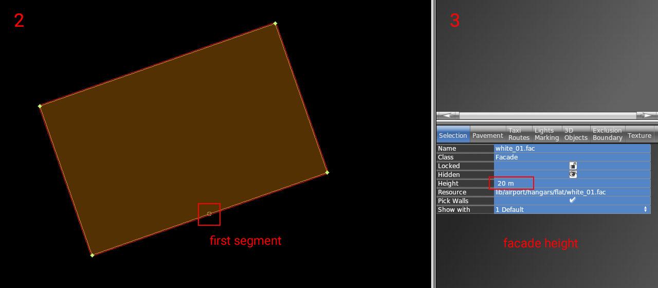
2 – Rotate the polygon (CTRL + R) until you get the first segment (marked with a small circle) to the place where the open doors should be. This is very important for future steps (aligning interior facade and doors)
3 – Set the desired height of the hangar (8, 10, 12, 16, 18, 22, 26, or 30). This is very important because the exact dimensions of openings and related parts may vary based on facade height.
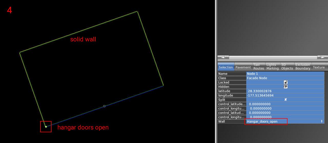
4 – Now set the correct wall types inside vertices. The most important is of course open doors (blue segment). For others, you can use whatever you need (solid walls, windows, etc).
5 – The exterior part is finished. Lock the shape to prevent unwanted edits (turn on the lock icon).
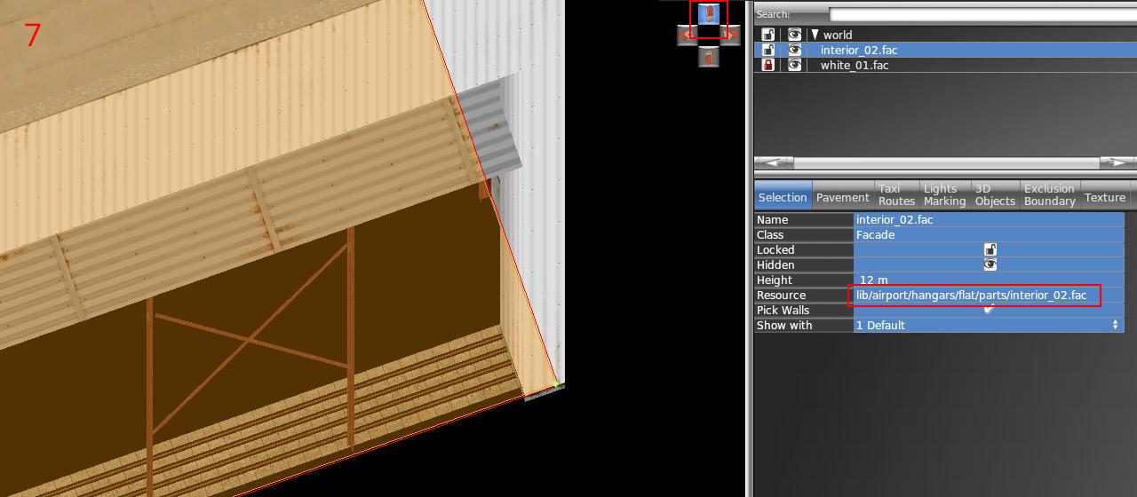
6 – Draw the hangar interior (lib/airport/hangars/flat/parts/interior_xx.fac) following the exact shape of the exterior. Use "snap to vertices" function. You should not break the exterior shape because it is locked.
7 – Make sure WED preview is turned on (menu View / Toggle Preview). Zoom to the hangar corner and use an appropriate isometric view.
8 – Set the corresponding height of the interior (7, 9, 11, 15, 17, 21, or 29). Note the height is one meter shorter than the exterior.
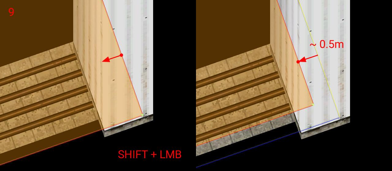
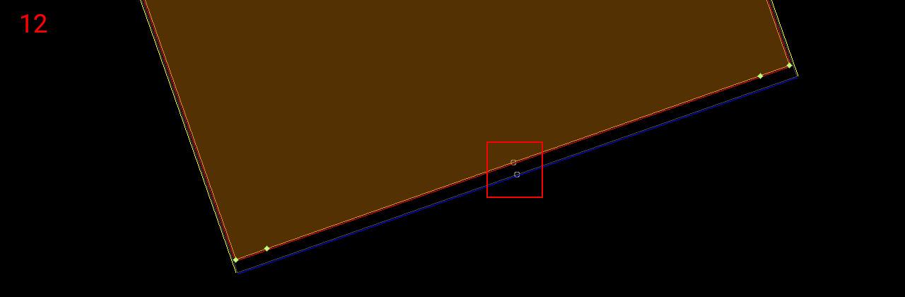
9 – With SHIFT pressed, drag the polygon toward the inside roughly 0.5 meters.
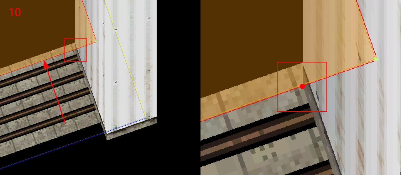
10 – Drag the segment with open doors towards the inside until reaches the end of the opening side. Make sure you're dragging only the single polygon segment (two vertices at a time), not the entire interior polygon.
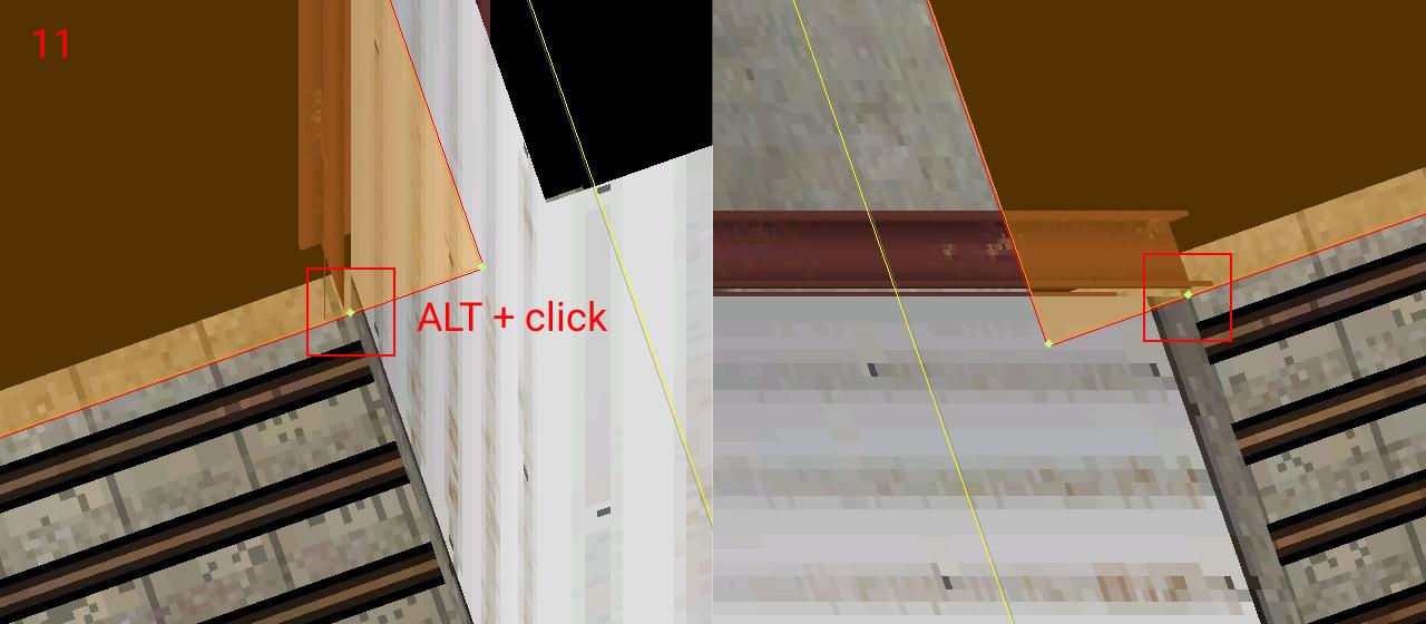
11 – Add a new vertex (using ALT + click) to the intersection of the polygon with the opening. Do the same on the opposite side of the doors (with an appropriate isometric view angle)
12 – Now rotate polygon segments (Ctrl + R) to get the first segment (white circle) to the corresponding position with the exterior facade polygon. This is very important for the alignment of both facades!
13 – Set the proper wall type to the opening (and other walls eventually). The Interior is done – you can lock the shape.
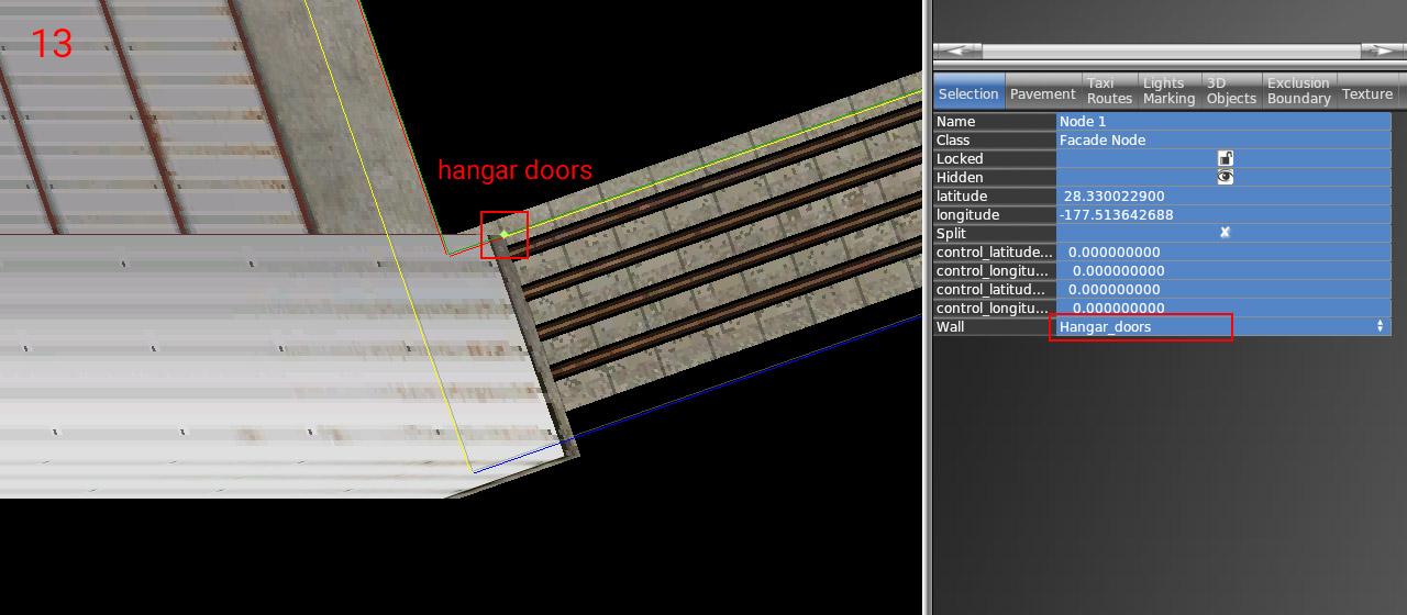
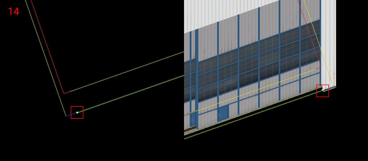
14 – Choose the door facade you want (lib/airport/hangars/flat/parts/hangar_door_xx.fac) and draw a single-segment polygon. Points should be placed exactly on the border of the exterior facade polygon (blue segment). Use the isometric preview to fit both endpoints.
15 – Set the corresponding height of the doors (matching hangar height levels – 8, 10, 12, 16, 18, 22, 26, or 30) and set the wall type to "Hangar_doors_open". You are done!
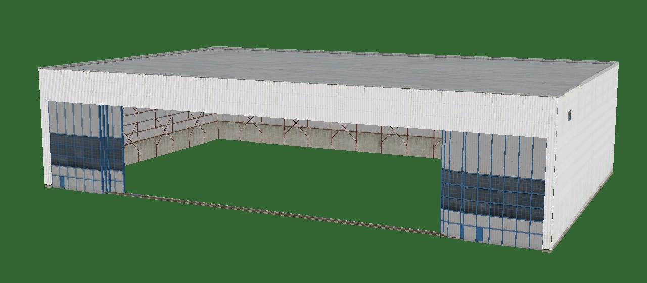
NOTE: All standalone door facades also have a wall with closed doors (Hangar_doors). This makes no sense in combination with the interior of course. But you can use it for making any combination of the exterior facade design and doors. In that case, you don't need to worry about the interior facade but everything else above is still true.
The old weather datarefs have been marked as deprecated in X-Plane 12 and replaced with two new sets. The old ones will remain in place but anything referencing them should be changed to use the new ones as soon as possible. The good news is that this should be fairly straightforward.
Previously the values returned in the datarefs were relative to the user's aircraft. This was fine for handling instrumentation but not ideal for working with the wider environment. There are now two similar sets of datarefs, one for the weather at the aircraft's exact position, and one for the surrounding region.
Aircraft
In general, all the old datarefs that lived under sim/aircraft/ have been moved under sim/weather/aircraft/ with very similar names. The only real thing to note here is that in some cases, units have changed. Also, all these aircraft-specific datarefs are read-only. This makes sense; the aircraft's immediate environment is a point sample from the regional weather.
Cloud, wind and turbulence datarefs are no longer represented by individual datarefs with an array-like notation, they are handled as real arrays. This means you should do proper array handling of these by querying the size of the array using XPLMGetDatavf() before your first read, and allocating enough space accordingly. Doing this will allow your code to continue to work with no changes if in the future the array size is changed. Temperature and wind arrays have already been increased to 13 elements from 3.
It's important to remember that the aircraft's immediate environment is a snapshot of a single point in a simulated 3D volume. This volume contains deliberate variations from whatever the base weather is, whether that's a fixed preset coming from the UI or a composite of available real-weather data if this is enabled. You should not, in other words, expect any value reported at the aircraft's position to exactly match any value you may see elsewhere that isn’t based on the aircraft’s position.
Region
New for X-Plane 12, the base weather that defines the aircraft's surrounding region is provided as a distinct set of datarefs under sim/weather/region/. Right now 'region' roughly corresponds to a square degree but this may vary in the future. The region base values determine a starting point for X-Plane's own weather simulation, which gets added on top. As with the aircraft's datarefs, this means that you should not expect any value returned in these datarefs to exactly match any value you see elsewhere since the weather at any given point is taken from the combination of the base weather and the weather simulation, not the starting data for that simulation.
Atmospheric Altitude Levels
Atmospheric temperatures are defined at preset altitudes which can be found in sim/weather/region/atmosphere_alt_levels_m . If you are working with temperatures aloft, please use the altitudes given in this array and don't hard-code them. The altitudes, or the number of layers, may change.
Modifying the Region
Most of the regional datarefs are writeable, meaning that you can use these to change the weather in a large volume surrounding the user's aircraft.
sim/weather/region/change_mode
This controls X-Plane's internal weather simulation, when used with static weather, by setting a general trend over time.
sim/weather/region/variability_pct
This controls the internal weather simulation's variability for those parts which use random noise to generate variation. The base weather also varies with distance from a given reference point. Typically the reference point would be the selected airport if you use the UI to select a weather preset, for example.
sim/weather/region/update_immediately
When this is non-zero, any changes to any regional dataref except clouds will take place immediately. Otherwise, the changes will start to fade in over a short period of time, currently 1-2 minutes. Clouds are handled a little differently because there is a delay between the cloud data being determined and the results of the GPU-based cloud simulation being returned. Even with update_immediately set to true, clouds will generally take a minute or so to update to the new values. When you absolutely, positively got to kill every cumulonimbus in the room, you can use the sim/operation/regen_weather command to trigger an immediate full reset of the current weather.
API Access
For simpler access if you are using a programming language that can use it, the X-Plane SDK contains some basic weather data access functions. These allow you to get a weather snapshot – that is, the equivalent of the aircraft datarefs, the output of the base weather plus the weather simulation – at a specific point.
While you are free to request weather for distant locations, the accuracy of the data returned will drop significantly outside of the current region. Errors are reported via the standard XPLMSetErrorCallback() mechanism.
X-Plane 12 features a 3-D HUD – besides drawing HUD markings on top of the 3-d scene, the HUD aligns to the world in 3-d with the same parallax error that a real HUD would have, and looks “far away” to a user in VR.
The HUD consists of three separate authoring elements:
An area of the aircraft’s 3-d panel texture that has HUD markings.
A 3-d mesh in an aircraft attached object with appropriate objects, that will serve as the HUD glass. The HUD image will only appear when the glass covers the screen space area in front of where the pilot “perceives” the HUD to be.
Plane-Maker settings to calibrate the 3-d HUD’s alignment.
Setting Up the HUD in Plane-Maker
Plane-Maker’s viewpoint cockpit screen contains a section “3-D HUD” that requires three types of information:
The field of view angles of the edge of the HUD glass. You may need to calculate these in your 3-d model – it is the number of degrees to the left, right, up and down from from the pilot looking straight ahead at the default pilot viewpoint.
The pixel position on the 3-d texture panel that the HUD image will be taken from. The lower left is 0,0, and the unit is pixels. You will be able to see this rectangle in the panel editor to validate that it is correctly set up, but it must be changed in the viewpoint cockpit screen.
The panel region. If your 3-d cockpit uses panel regions, pick the region number for the HUD here. If your aircraft does not use panel regions, you should leave this as the default “0” value.
Creating the HUD Graphics
In the 3-d panel editor, click the HUD icon in the upper right button bar (just to the left of the “2-D” icon) to view the HUD preview lines. If the panel is set up with a 3-d HUD, you will see:
A cyan box showing the edge of the HUD’s image and
A HUD ladder showing the horizontal center, horizon, and 2.5 degree vertical increments.
You can use these queue marks to calibrate your HUD graphics.
⚠️ WARNING: as of X-Plane 12.0.8 the “2-d” HUD instruments only work in the 2-d HUD, and the “3-d” HUD instruments only work in the 3-d HUD. We recommend using generic instruments for the 3-d HUD.
Setting Up the 3-d HUD Object
The 3-d HUD needs a glass element in an object, with a special attribute
    ATTR_hud_glass
    TRIS	36 18
    TRIS	54 18
  ATTR_hud_reset
Steps to Debug The HUD
First, confirm the HUD image is present by using the texture browser to view the night panel texture.
Second, confirm the HUD glass is present by temporarily removing the HUD glass attributes and giving it a debug color texture.
New 3D trees in X-Plane consist of two main parts.
The first part of a tree definition is a 2-d billboard side view of the tree. These operate almost identically to X-Plane 11 trees. In X-Plane 12, the side billboard always faces the camera and there is only one per tree.
The second part is one or more 3-d models of the tree that are used for close up rendering. X-Plane dynamically animates the 3-d model based on wind parameters.
X-Plane automatically uses the 3-d model of the tree for close rendering and transitions to the 2-d billboard for far views for performance.
The two parts of the tree use separate texture and materials – the 2-d textures and material is shared by all 2-d billboards in the .for file; the 3-d textures and material is shared by all 3-d models in the .for file.
This guide requires some basic Blender knowledge like adding vertex groups and weight painting.
Textures
Both parts use separate textures – one for billboards and another for 3D parts. This is also the main prerequisite – all billboards and all 3D parts for all trees (all species) within a single *.for must be in a single texture sheet. A typical pair of textures may look like this:
X-Plane 12 offers a new type of shader called translucent. It was designed specifically for 3D vegetation. Unlike a typical PBR shader, it has a different usage of the normal map blue channel. Instead of metallic property, it determines translucency. White color means fully translucent (leaves) and black means no translucent (solid parts – trunk). Here is what a typical normal map may look like:
Creating Trees in Blender
In Blender, all parts are organized in a hierarchy and in collections by strict rules. A single tree consists of three (or more) parts. The top-level object is an empty wrapper (Its name is used for the tree name on export). This parent wrapper must have two child objects – a billboard (single vertical quad) and a 3D tree (mesh object).
Each tree can have up to three 3D meshes. The reason is more per-tree LODs that can be additive. The typical use is: the first LOD mesh (0 to 500 m) has all triangles that are facing upward. The second LOD for a shorter distance (0 to 100 m) has all triangles that are facing towards the ground and thus don’t need to be visible for a bigger distance (bottom of branches). This is highly recommended for better performance, in particular when using high polycount on 3D meshes.
Trees are organized into forests using collections and each forest needs two levels. The top-level collection (right under the Scene root collection) is the forest itself. It consists of nothing but other collections. Those collections represent forest layers and all names must start with a numeric value (01, 02, 01-conifers, etc). This value is used as a tree layer index on the export. Obviously, all trees (with all their parts) must belong to some “layer” collection.
Parameters
All important parameters in Blender can be found in the properties editor but they’re spread across various tabs. All parts of a tree must be organized in the proper hierarchy and collection in order to get the options tab visible.
Global forest options can be found on the scene tab. Besides the main “Export” button the most important parameters here are the file name used on export, tree spacing, and global LOD distance. A separate tab for each existing root collection is shown. A collection is treated as a separate *.for on export once it has some filename entered.
The tree root object (empty wrapper) has all options on the objects tab. The “Weighted Importance” value is a relative occurrence of the tree within a forest layer. “Max tree height” is the size limit of the tree. The minimum height is determined from the real size of the tree billboard (in other words, trees are prepared in Blender in their minimum size).
3D tree mesh-specific options are on the object data tab. 3D tree mesh LOD values are set to 0 and 500 by default. This is also the recommended value for all trees that are intended to cast shadows because 500 meters is currently the default max shadow distance in X-Plane. Shorter distances might cause popping shadow artifacts, but for some types of meshes it is not important, such as bottom facing geometry.
In addition, both billboards and 3D meshes have material options on the material tab. It is recommended to use blend hash and normal translucency mode for both materials.
Adding Wind Effects
3D trees can sway in X-Plane’s dynamic wind. In order to do so the mesh needs additional vertex data. In Blender we have three vertex weight data channels: w_stiffness, w_edge_stiffness, and w_phase. These names are mandatory and case sensitive!
The stiffness channel (w_stiffness) is used to displace mesh vertices horizontally in the wind direction. The maximum distance of displacement (in meters) is defined by the stiffness parameter on the mesh data tab. It is a multiplier of the vertex data value.
Edge stiffness (w_edge_stiffness) is used to displace mesh vertices vertically (vertical oscillation or swaying).
Phase data (w_phase) is used to shift various branches’ movement in time. This can avoid uniformity in the look of the whole tree’s movement.
Stiffness and edge stiffness data might look very similar in most cases. Maximum weight value is on the tip of the branch and zero near the trunk. Phase data is different however. The whole branch usually has the same weight (any value in range 0 – 1).
On top of that the whole tree is bent by wind. This bend is calculated automatically from the ground to the top of the tree. The stronger the wind, the greater the bend at the top of the tree. There is a calibration value on the mesh data tab that can tweak the total amount according to tree height.
The default value of 1.0 is calibrated for a 10 meters tall tree. This value might change on the tree shape and the artist’s desires however. Here are a few examples:
10 m tree 1.0
20 m tree 0.5
30 m tree 0.3
5 m tree 1.6
Rock 0.0 (no bend)
Seasons
At this time the exporter has no automatic support for creation of seasons. It has to be done manually. To do so, make a copy of final *.for and change the texture to a different season variant. More info about seasons in different document (link?).
Tips & Tricks
The exporter is still in a very raw stage. Code isn’t error proof so you have to follow strict rules to avoid errors on export.
All parameters in the Blender UI have a tooltip with descriptions.
It is recommended to use one forest per one Blender scene.
Everything except proper forest collections must be turned off (excluded from View Layer) on export time.
Try to avoid extremely high polycounts. A typical big tree mesh can have 1000 – 2000 triangles, or 3000 – 4000 for very big, old trees.